Optimizing Genomic Prediction: A Practical Guide to Parameter Tuning for Enhanced Accuracy and Efficiency
This article provides a comprehensive guide to parameter tuning for genomic prediction models, a critical process for enhancing the accuracy and efficiency of breeding values in biomedical and agricultural research.
Optimizing Genomic Prediction: A Practical Guide to Parameter Tuning for Enhanced Accuracy and Efficiency
Abstract
This article provides a comprehensive guide to parameter tuning for genomic prediction models, a critical process for enhancing the accuracy and efficiency of breeding values in biomedical and agricultural research. Tailored for researchers and drug development professionals, it covers foundational principles, advanced methodological applications, strategic optimization techniques for troubleshooting common issues, and robust validation frameworks for model comparison. By synthesizing the latest research, this resource offers actionable strategies to navigate the complexities of model configuration, from selecting core algorithms to integrating multi-omics data, ultimately empowering scientists to build more reliable and powerful predictive models.
Core Principles and Key Parameters in Genomic Prediction
Defining Genomic Prediction and the Critical Role of Parameter Tuning
Defining Genomic Prediction
What is Genomic Prediction? Genomic Prediction (GP) is a methodology that uses genome-wide molecular markers to predict the additive genetic value, or breeding value, of an individual for a particular trait [1]. The core principle is that variation in complex traits results from contributions from many loci of small effect [1]. By using all available markers simultaneously without applying significance thresholds, GP sums these small additive genetic effects to estimate the total genetic merit of an individual, even for traits not yet observed [1].
What are its Primary Goals and Applications? The primary goal is to accelerate genetic improvement in plant and animal breeding by enabling selection of superior parents earlier in the lifecycle, thereby shortening breeding cycles and reducing costs [2] [1] [3]. In evolutionary genetics, GP models can predict the genetic value of missing individuals, understand microevolution of breeding values, or select individuals for conservation purposes [1]. More recently, its application has expanded to predict the performance of specific parental crosses, optimizing selection further [3].
Main Methodological Categories and Their Parameters
Genomic prediction methods can be divided into three main categories, each with distinct underlying assumptions and tuning parameters [2].
| Category | Description | Key Methods | Critical Parameters |
|---|---|---|---|
| Parametric | Assumes marker effects follow specific prior distributions (e.g., normal distribution). | GBLUP, BayesA, BayesB, BayesC, Bayesian LASSO (BL), Bayesian Ridge Regression (BRR) [2] [1]. | Prior distribution variances, shrinkage parameters [1]. |
| Semi-Parametric | Uses kernel functions to model complex, non-linear relationships. | Reproducing Kernel Hilbert Spaces (RKHS) [2] [4]. | Kernel type (e.g., Linear, Gaussian), kernel bandwidth/parameters [4]. |
| Non-Parametric | Makes fewer assumptions about the underlying distribution of marker effects; often machine learning-based. | Random Forest (RF), Support Vector Regression (SVR), Gradient Boosting (e.g., XGBoost, LightGBM) [2]. | Number of trees/tree depth, learning rate, number of boosting rounds, subsampling ratios. |
Benchmarking Performance and the Impact of Tuning
The predictive performance of different methods varies significantly based on the species, trait, and genetic architecture. Systematic benchmarking is essential for objective evaluation [2].
Comparative Performance of Different Methods A benchmarking study on diverse species revealed the following performance and computational characteristics [2]:
| Model Type | Example Methods | Mean Predictive Accuracy (r) | Relative Computational Speed | Relative RAM Usage |
|---|---|---|---|---|
| Parametric | Bayesian Models | Baseline | Baseline | Baseline |
| Non-Parametric | Random Forest | +0.014 | ~10x faster | ~30% lower |
| Non-Parametric | LightGBM | +0.021 | ~10x faster | ~30% lower |
| Non-Parametric | XGBoost | +0.025 | ~10x faster | ~30% lower |
Note: Predictive accuracy gains are relative to Bayesian models. Computational advantages do not account for hyperparameter tuning costs [2].
Choosing the Right Model and Tuning Strategy The optimal model depends on the genetic architecture of the trait:
- Parametric models like GBLUP/ridge regression are often accurate and fast for traits where a normal distribution of marker effects is a reasonable approximation, which is common in breeding populations with extensive linkage disequilibrium [1].
- Variable selection models (e.g., BayesB, LASSO) can be superior when individuals are less related and populations are polymorphic at some large-effect loci, as their priors allow some marker effects to be estimated as zero [1].
- Non-parametric/Machine Learning models show modest but significant gains in accuracy and major computational advantages for model fitting, though they require careful hyperparameter tuning [2].
- Kernel Methods (e.g., RKHS) are particularly powerful for capturing complex non-linear patterns and epistatic interactions that linear models might miss [4]. Tuning the kernel function and its parameters (e.g., the bandwidth in a Gaussian kernel) is critical for performance [4].
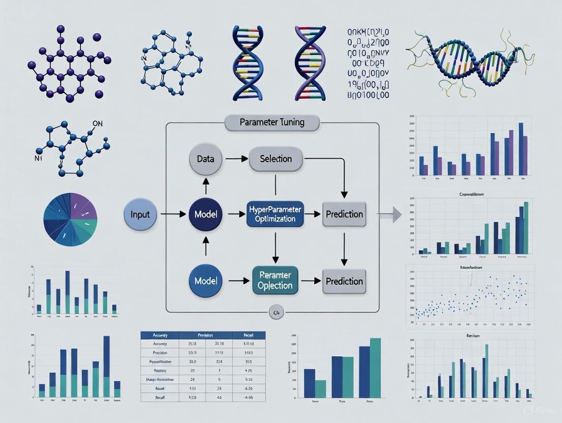
A Workflow for Genomic Prediction and Parameter Tuning
The following diagram illustrates the general workflow for developing a genomic prediction model, highlighting the iterative process of parameter tuning.
Essential Research Reagent Solutions
The table below lists key resources and tools used in modern genomic prediction research.
| Resource/Tool | Function in Genomic Prediction Research |
|---|---|
| EasyGeSe [2] | A curated collection of datasets from multiple species for standardized benchmarking of genomic prediction methods. |
| GPCP Tool [3] | An R package and BreedBase resource for predicting cross-performance using additive and dominance effects. |
| BreedBase [3] | An integrated platform for managing breeding program data, which hosts tools like GPCP. |
| sommer R Package [3] [5] | An R package used for fitting mixed models, including those for genomic prediction with complex variance-covariance structures. |
| AlphaSimR [3] | An R package for simulating breeding programs and genomic data, used to test methods and predict outcomes. |
Frequently Asked Questions (FAQs) and Troubleshooting
Q1: Why is parameter tuning so critical in genomic prediction? Parameter tuning is essential because the predictive performance of a model is highly sensitive to its hyperparameters. For instance, in machine learning models like gradient boosting, the learning rate and tree depth control the model's complexity and its ability to learn from data without overfitting. In kernel methods like RKHS, the kernel bandwidth determines the smoothness of the function mapping genotypes to phenotypes [4]. Inappropriate parameter values can lead to underfitting (failing to capture important patterns) or overfitting (modeling noise in the training data), both of which result in poor predictive accuracy on new, unseen genotypes.
Q2: My genomic prediction model is overfitting. How can I address this? Overfitting typically occurs when a model is too complex for the amount of data available.
- Increase Regularization: Most methods have regularization parameters. For parametric Bayesian models, this is controlled by the prior variance; for machine learning models like XGBoost, parameters like
gamma,lambda, andalphapenalize complexity. For kernel methods, a regularization parameter balances fit and smoothness [4]. - Reduce Model Complexity: Simplify your model by reducing the number of parameters (e.g., shallower trees in random forest, fewer components in a model).
- Gather More Data: If possible, increase the size of your training population.
- Use Cross-Validation: Rigorously use cross-validation to evaluate the true predictive performance and guide your tuning process, ensuring your model generalizes beyond the training set [1].
Q3: What is the practical impact of choosing a non-linear kernel over a linear one? A linear kernel assumes a linear relationship between genotypes and the phenotype. In contrast, non-linear kernels (e.g., Gaussian, polynomial) can capture more complex patterns, including certain types of epistatic (gene-gene interaction) effects [4]. The practical impact is that for traits with substantial non-additive genetic variance, a well-tuned non-linear kernel can provide higher prediction accuracy. However, this comes at the cost of increased computational complexity and the need to tune the additional kernel parameter (e.g., bandwidth) [4].
Q4: I'm getting an error with the predict.mmer function in the sommer R package. What should I do?
This is a known issue that users have encountered. The package developer has noted that the predict function for mmer objects can be unstable and has recommended two potential solutions [5]:
- Use the
mmec()function: Consider refitting your model using themmec()function instead ofmmer, and then use the correspondingpredict.mmec()function, which is more robust. - Use
fitted.mmeras a workaround: As an interim solution, you can usefitted.mmer(your_model)$dataWithFittedto obtain fitted values [5]. The developer is working on unifying the two functions in a future release.
Frequently Asked Questions
1. What are the fundamental differences between GBLUP, Bayesian, and Machine Learning models in genomic prediction?
The core difference lies in how they handle marker effects and genetic architecture.
- GBLUP: Uses a genomic relationship matrix (G-matrix) to model the genetic similarity between individuals, implicitly assuming all markers contribute equally to the trait (infinitesimal model) [6] [7].
- Bayesian Methods: Assume each marker can have its own effect, with specific prior distributions (e.g., BayesA, BayesB, BayesC) that allow for variable selection and unequal marker variances, better suited for traits influenced by a few major genes [8] [9].
- Machine Learning (ML): Non-parametric models like Deep Learning or Random Forest that flexibly learn complex, non-linear patterns and interactions from the data without strong pre-specified assumptions about the underlying genetic architecture [7] [10].
2. My GBLUP model performance is plateauing. What are the first parameters I should investigate tuning?
First, examine if the assumption of equal marker variance is limiting your predictions. Advanced tuning strategies include:
- Constructing a Weighted GBLUP (wGBLUP): Instead of a standard G-matrix, weight markers by their estimated effects (e.g., from an initial Bayesian analysis) to create a trait-specific relationship matrix. This can account for the unequal genetic variance of different genomic regions [6].
- Incorporating Non-Additive Effects: Build additional relationship matrices for dominance and epistasis (e.g., via Hadamard products of the additive G-matrix) and include them in your model to capture non-linear genetic effects [11] [12].
3. When should I choose a complex Deep Learning model over a conventional method like GBLUP?
Deep Learning excels when you have a large training population (e.g., >10,000 individuals) and suspect the trait is governed by complex, non-linear interactions (epistasis) that linear models cannot capture [11] [10]. For smaller datasets or traits with a predominantly additive genetic architecture, conventional methods like GBLUP or Bayesian models often provide comparable or superior performance with less computational cost and complexity [7] [10]. A hybrid approach, like the deepGBLUP framework, which integrates deep learning networks to estimate initial genomic values and a GBLUP framework to leverage genomic relationships, can sometimes offer the best of both worlds [11].
4. What are the common pitfalls when applying Machine Learning to genomic data, and how can I avoid them?
Common pitfalls and their solutions are summarized in the table below.
Table: Common Machine Learning Pitfalls in Genomics and Mitigation Strategies
| Pitfall | Description | Mitigation Strategy |
|---|---|---|
| Distributional Differences | Training and prediction sets come from different biological contexts or technical batches (e.g., different breeds, sequencing platforms) [13]. | Use visualization and statistical tests to detect differences. Apply batch correction methods or adversarial learning [13]. |
| Dependent Examples | Individuals in the dataset are genetically related, violating the assumption of independent samples [13]. | Use group k-fold cross-validation where related individuals are kept in the same fold. Employ mixed-effects models that account for covariance [13]. |
| Confounding | An unmeasured variable creates spurious associations between genotypes and phenotypes (e.g., population structure) [13]. | Include principal components of the genomic data as covariates in the model to capture and adjust for underlying structure [13]. |
| Leaky Preprocessing | Information from the test set leaks into the training set during data normalization or feature selection, causing over-optimistic performance [13]. | Perform all data transformations, including feature selection and scaling, within the training loop of the cross-validation, completely independent of the test set [13]. |
5. How can I systematically evaluate and compare the performance of different genomic prediction models?
A robust evaluation requires a standardized machine learning workflow:
- Cross-Validation (CV): Use k-fold CV to repeatedly split data into training and testing sets, ensuring the performance metric is an average over multiple partitions. For genomic data, use group k-fold CV to keep related individuals together and prevent overestimation [14].
- Hyperparameter Tuning: For each model, perform an inner cross-validation loop on the training set to find the optimal hyperparameters (e.g., learning rate for DL, shrinkage parameters for Bayesian models) [14].
- Performance Metrics: Use appropriate metrics for your trait type. For continuous traits, use Mean Square Error (MSE) or prediction accuracy (correlation between predicted and observed values). For binary traits, use area under the receiver operating characteristic curve (AUC) [14] [12].
Troubleshooting Guides
Guide 1: Troubleshooting GBLUP and Related Mixed Models
Problem: Low prediction accuracy, potentially due to oversimplified model assumptions.
Table: GBLUP Experimental Parameters and Tuning Guidance
| Parameter / Component | Description | Tuning Guidance & Common Protocols |
|---|---|---|
| Genomic Relationship Matrix (G) | A matrix capturing the genetic similarity between individuals based on their markers [6]. | Standardize genotypes to a mean of 0 and variance of 1 before calculating G. The vanilla G assumes all markers have equal variance. |
| Weighted GBLUP (wGBLUP) | An advanced G-matrix where SNPs are weighted by their estimated effects to reflect unequal variance [6]. | Protocol: 1) Run a Bayesian method (e.g., BayesA) on the training data. 2) Use the posterior variances of SNP effects as weights. 3) Construct a new, weighted G-matrix. 4) Refit the GBLUP model. This often outperforms standard GBLUP when trait architecture deviates from the infinitesimal model [6]. |
| Non-Additive Effects | Genetic effects not explained by the simple sum of allele effects, such as dominance and epistasis [11]. | Protocol: Construct separate relationship matrices for dominance (GD) and epistasis (GE). For epistasis, GE is often computed as the Hadamard product of the additive G-matrix with itself [11] [12]. Include these as random effects in a multi-kernel model: y = μ + Z<sub>a</sub>u<sub>a</sub> + Z<sub>d</sub>u<sub>d</sub> + Z<sub>e</sub>u<sub>e</sub> + e. |
The following diagram illustrates a recommended workflow for developing an advanced GBLUP model.
Guide 2: Troubleshooting Bayesian Models
Problem: Model is computationally intensive, slow to converge, or results are sensitive to prior choices.
Table: Bayesian Model Families and Tuning Strategies
| Model / Prior | Description | Tuning Focus & Computational Notes |
|---|---|---|
| BayesA | Each SNP has its own effect, sampled from a Student's t-distribution. Shrinks small effects but allows large ones [9]. | Tuning the degrees of freedom and scale parameters of the t-distribution is crucial. Computationally intensive via MCMC. |
| BayesB | A variable selection model: a proportion (π) of SNPs have zero effect; the rest have effects from a t-distribution [8] [9]. | The π parameter (proportion of SNPs with zero effect) is critical. It can be pre-specified or estimated from the data (BayesBπ). MCMC sampling can be slow. |
| BayesC & BayesCπ | Similar to BayesB, but non-zero effects are sampled from a single normal distribution [8]. | Simpler than BayesB. In BayesCπ, the proportion π is estimated. Often offers a good balance between flexibility and computational stability. |
| Bayesian LASSO (BL) | Uses a Laplace (double-exponential) prior to strongly shrink small effects to zero [9]. | The regularization parameter (λ) controls the level of shrinkage. It can be assigned a hyperprior to be estimated from the data. |
Actionable Protocol: Implementing an Efficient Bayesian Analysis
- Choice of Prior: Start with BayesCÏ€ as a default for its balance of variable selection and computational efficiency. Use more complex priors (e.g., BayesB) if you have strong evidence of a trait controlled by very few QTL [8].
- Computational Speed-up: For large datasets, consider fast Expectation-Maximization (EM) algorithms (e.g., fastBayesA) that approximate the posterior mode instead of full MCMC sampling, significantly reducing computation time [8] [9].
- Convergence Diagnosis: When using MCMC, always run multiple chains with different starting values. Use diagnostics like the Gelman-Rubin statistic to assess convergence. Visually inspect trace plots to ensure the chain is mixing well and is not stuck [9].
Guide 3: Troubleshooting Machine Learning Models
Problem: A complex ML model (e.g., Deep Learning) is underperforming a simple linear model.
Actionable Protocol: A Standardized ML Workflow for Genomics Adhering to a rigorous workflow is key to successfully applying ML in genomics.
- Data Preprocessing and Splitting: Standardize genotype data. Use Group K-Fold Cross-Validation to split data, ensuring that genetically related individuals are not split across training and test sets, which prevents data leakage and over-optimistic performance [13] [14].
- Hyperparameter Tuning: Conduct an inner cross-validation loop within the training set to find the optimal model settings. For example:
- Model Training and Evaluation: Train the model on the entire training set with the best hyperparameters. Make final predictions on the untouched test set and calculate your performance metrics (e.g., MSE, accuracy). Repeat this process for all folds in the outer loop to get a robust estimate of model performance [14].
The Scientist's Toolkit
Table: Essential Research Reagents and Software for Genomic Prediction
| Item Name | Type | Function / Application |
|---|---|---|
| PLINK | Software | A core tool for genome association analysis. Used for quality control (QC) of SNP data, filtering by minor allele frequency (MAF), and basic data management [11]. |
| GBLUP | Software / Model | Available in many mixed-model software packages. Used for genomic prediction assuming an infinitesimal model and for constructing genomic relationship matrices [6] [7]. |
| BGLR R Package | Software | A comprehensive R package for implementing a wide range of Bayesian regression models, including the entire "Bayesian Alphabet" (BayesA, B, C, LASSO, etc.) [8]. |
| SKM R Library | Software | A user-friendly R library for implementing seven common statistical machine learning methods (e.g., Random Forest, SVM, GBM) for genomic prediction, with built-in tools for cross-validation and hyperparameter tuning [14]. |
| Sparse Kernel Methods | Method | A class of kernel methods (e.g., Gaussian, Arc-cosine) that can capture complex, non-linear patterns and epistatic interactions more efficiently than deep learning for some datasets [12]. |
| Locally-Connected Layer (LCL) | Method | A deep learning layer used in networks like deepGBLUP. Unlike convolutional layers, it uses unshared weights, allowing it to assign marker effects based on their distinct genomic loci, which is more biologically appropriate for SNP data [11]. |
| N6-(2-Phenylethyl)adenosine | N6-(2-Phenylethyl)adenosine, MF:C18H21N5O4, MW:371.4 g/mol | Chemical Reagent |
| 10-Formyl-7,8-dihydrofolic acid | 10-Formyl-7,8-dihydrofolic acid, CAS:25377-55-3, MF:C20H21N7O7, MW:471.4 g/mol | Chemical Reagent |
Frequently Asked Questions (FAQs)
1. How does trait heritability influence the required size of my reference population? Trait heritability ((h^2)) is a primary factor determining the achievable accuracy of Genomic Estimated Breeding Values (GEBVs). For traits with low heritability, a larger reference population is required to achieve a given level of prediction accuracy. Simulation studies in Japanese Black cattle showed that for a trait with a heritability of 0.1, a reference population of over 5,000 animals was needed to achieve a high accuracy. In contrast, for a trait with a heritability of 0.5, a similar accuracy could be reached with a smaller population [15].
2. Is there a point of diminishing returns for marker density in genomic selection? Yes, genomic prediction accuracy typically improves as marker density increases but eventually reaches a plateau. Beyond this point, adding more markers does not meaningfully improve accuracy, allowing for cost-effective genotyping strategies.
- In mud crab, accuracy plateaued after using approximately 10,000 SNPs [16].
- In Pacific white shrimp, the accuracy saw diminishing returns after about 3,200 SNPs [17].
- In meat rabbits, a density of 50K SNPs was established as a suitable baseline [18].
- In olive flounder, using 3,000–5,000 randomly selected SNPs resulted in predictive ability similar to using 50,000 SNPs [19].
3. What is the minimum recommended size for a reference population? The minimum size is context-dependent, varying with the species' genetic diversity and the trait's heritability. However, some studies provide concrete guidelines:
- Mud crab: A reference population of at least 150 individuals was identified as a minimum standard for growth-related traits [16].
- Japanese Black cattle: For carcass traits (with (h^2) ~0.29-0.41), a reference population of 7,000–11,000 animals was sufficient to achieve accuracies (0.73–0.79) comparable to those from progeny testing [15].
- General finding: The accuracy of Genomic Selection (GS) consistently improves as the reference population size expands, as demonstrated in mud crabs where increasing the size from 30 to 400 individuals led to significant accuracy gains [16].
4. Do different genomic prediction models perform differently? The choice of model can be important, but studies across various species often find that the differences in prediction accuracy between common models (e.g., GBLUP, BayesA, BayesB, BayesC, rrBLUP) are often quite small [16] [17]. GBLUP is frequently noted for its computational efficiency and unbiased predictions when the reference population is sufficiently large [16]. Furthermore, multi-trait models can significantly improve accuracy for genetically correlated traits compared to single-trait models [18].
Table 1: The Interplay of Heritability, Reference Population Size, and Genomic Prediction Accuracy (Based on Simulation in Japanese Black Cattle)
| Trait Heritability ((h^2)) | Reference Population Size | Expected Prediction Accuracy |
|---|---|---|
| 0.10 | 5,000 | ~0.50 |
| 0.25 | 5,000 | ~0.65 |
| 0.50 | 5,000 | ~0.78 |
| 0.10 | 10,000 | ~0.58 |
| 0.25 | 10,000 | ~0.73 |
| 0.50 | 10,000 | ~0.84 |
Source: Adapted from [15]
Table 2: Observed Plateaus for Marker Density and Reference Population Size in Various Species
| Species | Trait Category | Marker Density Plateau | Minimum/Maximizing Reference Population Size |
|---|---|---|---|
| Mud Crab | Growth-related | ~10,000 SNPs [16] | Minimum: 150 [16] |
| Pacific White Shrimp | Growth | ~3,200 SNPs [17] | Not Specified |
| Japanese Black Cattle | Carcass | Not a primary focus | 7,000-11,000 for high accuracy [15] |
| Meat Rabbit | Growth and Slaughter | ~50,000 SNPs [18] | Not Specified |
Detailed Experimental Protocols
Protocol 1: Optimizing Marker Density and Reference Population Size
This protocol outlines a general experimental workflow to determine the optimal marker density and reference population size for a genomic selection program, as implemented in studies on species like mud crab and shrimp [16] [17].
1. Population, Phenotyping, and Genotyping:
- Population: Establish a population of individuals with recorded pedigrees, ensuring a wide genetic diversity representative of the breeding population.
- Phenotyping: Accurately measure the target trait(s) of interest (e.g., body weight, carapace length) on all individuals.
- Genotyping: Genotype the entire population using a high-density SNP array or sequencing (e.g., low-coverage whole-genome sequencing) to obtain a comprehensive set of genome-wide markers [16] [18].
2. Data Quality Control (QC) and Imputation:
- Perform stringent QC on the genotypic data using software like PLINK. Common filters include removing markers with a low minor allele frequency (e.g., MAF < 0.05), high missing genotype rates (e.g., >10%), and significant deviation from Hardy-Weinberg equilibrium [16] [15].
- Remove individuals with high missing genotype rates (e.g., call rate < 90%) [16].
- Impute any remaining missing genotypes using software such as Beagle [16] [15].
3. Genetic Parameter Estimation:
- Estimate the genomic heritability ((h^2)) of the trait using a genomic relationship matrix (GRM) and the GREML method implemented in software like GCTA [16].
- Estimate variance components to understand the proportion of phenotypic variance attributable to genetics.
4. Testing Marker Density:
- Create random subsets of SNPs from the full, high-quality dataset at various densities (e.g., 0.5K, 1K, 5K, 10K, 20K, up to the full set) [16] [17].
- For each density subset, perform genomic prediction using a chosen model (e.g., GBLUP) and a cross-validation scheme.
- Calculate the prediction accuracy (e.g., correlation between GEBV and observed phenotype in the validation population) for each density.
- Identify the density where accuracy plateaus, indicating the cost-effective optimum.
5. Testing Reference Population Size:
- Randomly sample subsets of individuals from the full dataset at various sizes (e.g., 50, 100, 200, 400) to act as reference populations [16].
- Use the remaining individuals as the validation population.
- For each reference population size, perform genomic prediction and calculate the prediction accuracy.
- Plot accuracy against reference population size to visualize the relationship and identify points of diminishing returns.
Protocol 2: Implementing a Multi-Trait Genomic Selection Model
This protocol describes the steps to implement a multi-trait GBLUP model, which can improve prediction accuracy for genetically correlated traits [18].
1. Data Preparation:
- Collect phenotypic records for multiple traits and genotypic data for all individuals in the reference population.
- Perform the same QC and imputation steps as in Protocol 1.
2. Variance-Covariance Estimation:
- Estimate the genetic variance for each trait and the genetic covariance between each pair of traits. This creates the genetic variance-covariance matrix (M). This can be done using REML methods.
3. Model Fitting:
- Fit a multi-trait linear mixed model. The model for two traits can be specified as:
[
\begin{bmatrix} \mathbf{y1} \ \mathbf{y2} \end{bmatrix} = \begin{bmatrix} \mathbf{X1} & \mathbf{0} \ \mathbf{0} & \mathbf{X2} \end{bmatrix} \begin{bmatrix} \mathbf{b1} \ \mathbf{b2} \end{bmatrix} + \begin{bmatrix} \mathbf{Z1} & \mathbf{0} \ \mathbf{0} & \mathbf{Z2} \end{bmatrix} \begin{bmatrix} \mathbf{a1} \ \mathbf{a2} \end{bmatrix} + \begin{bmatrix} \mathbf{e1} \ \mathbf{e2} \end{bmatrix}
]
where:
- (\mathbf{y}) is the vector of phenotypic values for the two traits.
- (\mathbf{X}) and (\mathbf{Z}) are design matrices for fixed and random effects, respectively.
- (\mathbf{b}) is the vector of fixed effects (e.g., sex, batch).
- (\mathbf{a}) is the vector of additive genetic effects, assumed to follow (N(0, \mathbf{M} \otimes \mathbf{G})), where (\mathbf{G}) is the genomic relationship matrix.
- (\mathbf{e}) is the vector of random residuals [18].
4. Prediction and Validation:
- Use the fitted model to predict GEBVs for all traits in the validation population.
- Validate the model using cross-validation and compare its accuracy to single-trait models.
Workflow and Logical Relationships
Research Reagent Solutions
Table 3: Essential Materials and Software for Genomic Prediction Experiments
| Item Name | Function / Application | Example Use Case |
|---|---|---|
| SNP Array | High-throughput genotyping platform for scoring thousands to hundreds of thousands of SNPs across the genome. | "Xiexin No. 1" 40K SNP array for mud crabs [16]; GGP BovineLD v4.0 for cattle [15]. |
| Low-Coverage Whole-Genome Sequencing (lcWGS) | A cost-effective method for genotyping by sequencing the entire genome at low depth, followed by imputation to a high-density variant set. | Genotyping in meat rabbits [18]. |
| PLINK | Software tool for whole-genome association and population-based linkage analysis; used for rigorous quality control of SNP data. | Filtering SNPs based on MAF, missingness, and HWE in cattle and shrimp studies [16] [17]. |
| Beagle | Software for phasing genotypes and imputing ungenotyped markers, crucial for handling missing data. | Imputing missing genotypes in mud crab and cattle studies [16] [15]. |
| GCTA | Software tool for Genome-wide Complex Trait Analysis; used for estimating genomic heritability and genetic correlations. | Estimating variance components and heritability using the GREML method [16]. |
| rrBLUP / BGLR R Packages | R packages providing functions for genomic prediction, including RR-BLUP and various Bayesian models. | Fitting GBLUP and Bayesian models in various species [19] [17]. |
| Genomic Relationship Matrix (GRM) | A matrix quantifying the genetic similarity between individuals based on marker data; foundational for many prediction models. | Constructed from all SNPs to estimate additive genetic variance in mixed models [16] [15]. |
Understanding the Impact of Genetic Architecture on Parameter Selection
Frequently Asked Questions (FAQs)
FAQ 1: How does genetic architecture influence the choice of a genomic prediction model? The genetic architecture of a trait—meaning the number of causal variants and the distribution of their effect sizes—is a primary factor in selecting an appropriate model.
- For highly polygenic architectures (many small-effect variants), models like gBLUP (Genomic Best Linear Unbiased Prediction) or rrBLUP (ridge regression BLUP) are recommended. These models assume all markers have a small, normally distributed effect, which is a robust and computationally efficient approximation for many complex traits [1] [20].
- For traits influenced by a few moderate- to large-effect variants alongside many small effects, variable selection models like BayesB, BayesC, or LASSO are often more accurate. These methods allow some marker effects to be shrunk to zero, better capturing a "sparse" genetic architecture [1] [20].
- A simple initial GWAS Manhattan plot can guide model selection. Traits showing a few "spiked" signals may benefit from variable selection models, while those with a diffuse, polygenic background are well-suited to gBLUP [20].
FAQ 2: Why does my genomic prediction model show low accuracy even when heritability is high? Low prediction accuracy can stem from a mismatch between your model's assumptions and the true genetic architecture, or from population structure [21].
- Architecture-Model Mismatch: Applying an additive, infinitesimal model (like G-BLUP) to a trait governed largely by epistatic (non-additive) interactions can result in poor accuracy. In such cases, models that explicitly account for interactions can improve performance [21].
- Population Structure: High prediction accuracy in breeding populations is often driven by high relatedness and linkage disequilibrium (LD) between individuals. In populations of unrelated individuals (e.g., human cohorts or diverse plant lines) with low LD, accuracy will naturally be lower unless the genetic architecture is explicitly accounted for in the model [21] [22].
- Training Population Composition: The relatedness between the calibration (training) and validation sets significantly impacts accuracy. Including progenitors in the training set can dramatically improve the accuracy of predicting progeny performance [22].
FAQ 3: What is the practical difference between GBLUP and Bayesian models like BayesB? The core difference lies in their prior assumptions about how marker effects are distributed.
- GBLUP/rrBLUP assumes a single, normal distribution for all marker effects. This is the infinitesimal model, where every marker contributes a small effect, and no markers are excluded [1].
- BayesB assumes a mixture distribution. A proportion of markers are assumed to have zero effect, while the rest have effects drawn from a normal or t-distribution. This makes it a variable selection model, which is more flexible for traits with large-effect loci [1].
Table 1: Key Factors Affecting Genomic Prediction Accuracy
| Factor | Impact on Prediction Accuracy | Key Finding |
|---|---|---|
| Trait Heritability | Positive correlation | Higher heritability generally enables higher prediction accuracy [22]. |
| Training Population Size | Positive correlation | Larger reference populations yield more accurate predictions [22]. |
| Relatedness & LD | Positive correlation | High relatedness and LD between training and target populations boost accuracy [21] [22]. |
| Genetic Architecture | Determines optimal model | Matching the model to the architecture (e.g., polygenic vs. sparse) is critical for maximizing accuracy [20] [21]. |
Troubleshooting Guides
Problem 1: Low Genomic Prediction Accuracy
Observation: The correlation between predicted and observed values in the validation set is low.
| Observation | Potential Cause | Options to Resolve |
|---|---|---|
| Low prediction accuracy in unrelated individuals | Mismatch between genetic architecture and model assumption; Low LD | 1. Perform a GWAS to visualize genetic architecture (e.g., Manhattan plot) [20]. 2. Switch from GBLUP to a variable selection model (e.g., Bayesian LASSO) if large-effect loci are detected [1] [21]. 3. Incorporate significant variants from GWAS into a customized relationship matrix for prediction [21]. |
| Accuracy drops when predicting progeny performance | Recombination breaks down marker-QTL phases; Selection changes allele frequencies | 1. Include the parents of the target progeny population in the training set [22]. 2. Re-train models each generation using the most recent data to maintain accuracy [22]. |
| Low accuracy for a trait with known high heritability | Model is unable to capture non-additive genetic effects | 1. Use models that explicitly account for epistatic interactions [21]. 2. Ensure the training population is sufficiently large and has power to detect the underlying architecture [21]. |
Problem 2: Selecting the Wrong Model for Your Trait's Genetic Architecture
Observation: Uncertainty about which genomic prediction model to apply for a novel trait.
Table 2: Genomic Prediction Model Selection Guide Based on Genetic Architecture
| Model Category | Example Models | Assumed Genetic Architecture | Best For Traits That Show... |
|---|---|---|---|
| Infinitesimal / Polygenic | GBLUP, rrBLUP | Many thousands of loci, each with a very small effect [1] | A "diffuse" Manhattan plot with no prominent peaks (e.g., human height) [20]. |
| Variable Selection | BayesB, BayesC, LASSO | A mix of zero-effect markers and markers with small-to-large effects [1] | A "spiked" Manhattan plot with a few significant peaks (e.g., some autoimmune diseases) [20]. |
| Flexible / Mixture | BayesR, DPR (Dirichlet Process Regression) | A flexible distribution that can adapt to various architectures, from sparse to highly polygenic [20] | An unknown or complex architecture, or when you want to avoid strong prior assumptions [20]. |
Diagnostic Strategy Flow:
- Visualize: Conduct a GWAS and examine the Manhattan plot for the trait [20].
- Classify: Categorize the architecture as "diffuse" (use GBLUP) or "spiked" (use variable selection).
- Test: Use cross-validation to compare the accuracy of 2-3 recommended models from the table above.
- Validate: Always validate the final model's predictive performance on an independent, untested dataset.
The Scientist's Toolkit: Research Reagent Solutions
Table 3: Essential Components for Genomic Prediction Studies
| Item | Function in Genomic Prediction |
|---|---|
| High-Density SNP Array / Whole-Genome Sequencing | Provides the genome-wide molecular marker data (genotypes) required to build the genomic relationship matrix (GRM) and estimate marker effects [1]. |
| Phenotyped Training Population | A set of individuals with accurately measured traits of interest. The size and genetic diversity of this population are critical for model accuracy [22]. |
| Genomic Relationship Matrix (GRM) | A matrix quantifying the genetic similarity between all pairs of individuals based on marker data. It is the foundational component of models like GBLUP [1]. |
| Linear Mixed Model (LMM) Software | Software packages (e.g., GCTA, BLR, BGLR) that implement various genomic prediction algorithms to estimate breeding values and partition genetic variance [1] [20]. |
| GLP-1 receptor agonist 11 | GLP-1 receptor agonist 11, CAS:2784590-83-4, MF:C31H31ClFN3O4, MW:564.0 g/mol |
| SPSB2-iNOS inhibitory cyclic peptide-1 | SPSB2-iNOS inhibitory cyclic peptide-1, MF:C35H56N12O14S2, MW:933.0 g/mol |
Experimental Protocols & Workflows
Detailed Methodology: Assessing Prediction Accuracy Across Generations
This protocol is based on a study in maritime pine [22] and is crucial for validating models in a breeding context.
1. Design the Reference Population:
- Select individuals covering multiple generations (e.g., G0 founders, G1 parents, G2 progeny).
- Use pedigree and phenotype information for pre-selection, aiming to control effective population size.
- Genotype all individuals using a high-density SNP array.
2. Define Calibration and Validation Sets:
- Within-Generation Validation: Split a single generation (e.g., G1) into training and testing sets to establish a baseline accuracy.
- Across-Generation (Progeny) Validation: Use earlier generations (G0 and G1) as the calibration set to predict the breeding values of the progeny generation (G2). This tests the model's practical utility.
3. Run Genomic Prediction Models:
- Apply multiple models (e.g., ABLUP-pedigree, GBLUP-markers, Bayesian LASSO) to the same calibration set.
- Use the models to generate Genomic Estimated Breeding Values (GEBVs) for the validation set.
4. Calculate Prediction Accuracy:
- For the validation set, calculate the correlation between the predicted GEBVs and the observed phenotypes (or pedigree-based EBVs).
- Compare accuracies between different models and validation designs to determine the most robust strategy.
Workflow Visualization
Diagram 1: Genetic Architecture Decision Workflow
Diagram 2: Genomic Prediction Experimental Process
Advanced Methods and Practical Implementation Strategies
Frequently Asked Questions (FAQs)
1. When should I choose GBLUP over a Bayesian model like BayesC for my genomic prediction task?
Your choice should be guided by the underlying genetic architecture of your trait and your computational resources.
- Opt for GBLUP when you are working with polygenic traits influenced by many genes with small effects. GBLUP assumes all markers contribute equally to the genetic variance and is highly robust across various scenarios. It is also computationally efficient and less prone to convergence issues [23] [24].
- Choose BayesC when you have prior knowledge or suspicion that the trait is influenced by a fewer number of quantitative trait loci (QTLs) with larger effects. BayesC performs variable selection by assuming that only a fraction of markers have a non-zero effect, which can be advantageous for traits with low to moderate numbers of QTLs [23] [24].
The table below summarizes the key differences to guide your selection:
| Feature | GBLUP | BayesC |
|---|---|---|
| Underlying Assumption | All markers have an effect, following an infinitesimal model [25]. | Only a fraction ((\pi)) of markers have a non-zero effect; performs variable selection [26]. |
| Best for Trait Architecture | Polygenic traits with many small-effect QTLs [24]. | Traits with a low to moderate number of QTLs or major genes [24]. |
| Computational Demand | Generally faster and less computationally intensive [27]. | More demanding, often requiring Markov Chain Monte Carlo (MCMC) methods [26]. |
| Impact of Heritability | Tends to perform more consistently across heritability levels; can be better for low-heritability traits [23]. | Prediction advantage can become more obvious as heritability increases [23]. |
2. How do factors like heritability and marker density affect prediction accuracy, and how can I optimize them?
Prediction accuracy is influenced by several factors, and understanding their interaction is key to optimizing your model.
- Heritability: Higher heritability generally leads to higher prediction accuracy for all models. GBLUP has been shown to be particularly robust for traits with low heritability, while Bayesian methods like BayesC may show a greater relative advantage as heritability increases [23].
- Marker Density: Increasing marker density typically improves accuracy by providing better genome coverage and capturing more causative variants [23]. However, the gain depends on the model and trait. For complex, polygenic traits, GBLUP with high-density markers is effective. When using sequence data with many non-causal variants, Bayesian variable selection models like BayesC can be more efficient at identifying the true signals [26].
The following workflow diagram outlines the decision process for configuring your model based on these factors:
3. My Bayesian model (e.g., BayesC) is running very slowly or failing to converge. What can I do?
Slow performance and convergence issues are common challenges with MCMC-based Bayesian models. Here are several troubleshooting steps:
- Verify Model Configuration: Ensure your prior distributions and the value of (\pi) (in BayesC) are appropriately set for your data. Misspecified priors can lead to poor mixing and slow convergence.
- Check Diagnostic Metrics: Use convergence diagnostics like (\hat{R}) (R-hat), which should be ≤ 1.01 for modern best practices, and examine trace plots to ensure chains are well-mixed and stationary [28].
- Consider Computational Shortcuts: For large datasets, especially those involving whole-genome sequence data, consider using Singular Value Decomposition (SVD). SVD can be applied to the genotype matrix to directly estimate marker effects for models like BayesC in a non-iterative, computationally efficient manner, achieving similar accuracies to traditional MCMC methods [26].
- Simplify the Model: If troubleshooting fails, a simpler model like GBLUP can be a robust alternative, especially for highly polygenic traits, and is much faster to compute [23] [25].
4. Are there alternatives to traditional regression models for genomic selection?
Yes, reformulating the problem can sometimes yield better results for specific breeding objectives.
- Binary Classification Approach: You can reformulate genomic selection as a binary classification problem. Instead of predicting a continuous breeding value, you classify individuals as "top" or "not top" performers based on a threshold (e.g., the 90th percentile or the performance of a check variety). Training a classification model this way can significantly increase sensitivity for selecting the best candidate lines [29].
- Machine Learning Models: Non-parametric methods like Random Forest, XGBoost, and LightGBM are also used. Benchmarking studies have shown they can offer modest gains in accuracy and major computational advantages in fitting time compared to some Bayesian methods, though they require careful hyperparameter tuning [27].
Experimental Protocols & Workflows
Standard Protocol for Implementing and Comparing GBLUP and BayesC
This protocol provides a step-by-step guide for a standard genomic prediction analysis, allowing for a fair comparison between GBLUP and BayesC.
1. Data Preparation and Quality Control
- Genotypic Data: Start with your raw genotype matrix. Perform quality control (QC) by filtering out markers with a high missing rate (e.g., >10-20%) and a low minor allele frequency (e.g., MAF < 0.05) [25]. Impute remaining missing genotypes using software like Beagle [27].
- Phenotypic Data: Collect and pre-process phenotypic records. Correct for fixed effects (e.g., herd, year, sex) if necessary, often by using Best Linear Unbiased Estimators (BLUEs) or de-regressed breeding values.
2. Model Training & Cross-Validation
- Population Splitting: Use a k-fold cross-validation (e.g., 5-fold) scheme. Randomly divide the population into k subsets. Iteratively use k-1 folds as the training set to estimate model parameters and the remaining fold as the validation set to assess accuracy [23] [25].
- Model Implementation:
- GBLUP: Fit the model by solving its mixed model equations (MMEs). The genomic relationship matrix (G) is calculated from the scaled and centered genotype matrix Z as G = ZZ' / m, where m is the number of markers [25].
- BayesC: Fit the model using an MCMC algorithm (e.g., Gibbs sampling). Specify prior distributions for the marker effects and the parameter (\pi). Run a sufficient number of iterations, discarding the initial iterations as burn-in.
3. Evaluation and Accuracy Calculation
- The primary metric for evaluation is the prediction accuracy, calculated as the correlation between the genomic estimated breeding values (GEBVs) and the observed (or corrected) phenotypic values in the validation set [25] [24].
The workflow for this protocol is visualized below:
The Scientist's Toolkit: Research Reagent Solutions
This table details key resources and datasets essential for benchmarking and implementing genomic prediction models.
| Resource / Solution | Function / Description | Relevance to Model Selection |
|---|---|---|
| EasyGeSe Database [27] | A curated collection of ready-to-use genomic and phenotypic datasets from multiple species (barley, maize, pig, rice, etc.). | Provides standardized data for fair benchmarking of new methods (e.g., GBLUP vs. BayesC) across diverse genetic architectures. |
| RR-BLUP / GBLUP R package [25] | An R package (e.g., rrBLUP) that provides efficient functions like mixed.solve() for implementing GBLUP and RR-BLUP models. |
Essential for the practical application of GBLUP, allowing estimation of breeding values and genomic heritability. |
| Stan or PyMC3 Software [28] | Advanced platforms that use Hamiltonian Monte Carlo (HMC) for efficient fitting of complex Bayesian models. | Useful for implementing custom Bayesian models like BayesC, though they require careful troubleshooting of MCMC diagnostics. |
| Beagle Imputation Software [27] | A software tool for phasing and imputing missing genotypes in genotype data. | A critical pre-processing step to ensure high-quality, complete genotype data for both GBLUP and Bayesian models. |
| Singular Value Decomposition (SVD) [26] | A matrix decomposition technique that can be applied to the genotype matrix. | A computational shortcut to enable fast, non-MCMC-based estimation for models like BayesC, especially with large WGS data. |
| PTP1B-IN-3 diammonium | PTP1B-IN-3 diammonium, MF:C12H13BrF2N3O3P, MW:396.12 g/mol | Chemical Reagent |
| Anti-inflammatory agent 31 | Anti-inflammatory agent 31, MF:C19H30O3, MW:306.4 g/mol | Chemical Reagent |
In the field of genomic prediction, the accurate selection and tuning of machine learning models are paramount for translating vast genomic datasets into meaningful biological insights and predictive models. Among the plethora of available algorithms, Kernel Ridge Regression (KRR) and Gradient Boosting, specifically through its advanced implementation XGBoost, have demonstrated exceptional performance in handling the complex, high-dimensional nature of genomic data. KRR combines the kernel trick, enabling the capture of nonlinear relationships, with ridge regression's regularization to prevent overfitting. In contrast, XGBoost employs an ensemble of decision trees, sequentially built to correct errors from previous trees, offering robust predictive power. However, the sophisticated process of hyperparameter tuning presents a significant barrier to their wider application in actual breeding and drug development programs. This technical support center provides targeted troubleshooting guides and detailed methodologies to empower researchers in overcoming these challenges, thereby accelerating breeding progress and enhancing predictive accuracy in genomic selection [30].
Troubleshooting Guides & FAQs
Q1: My Kernel Ridge Regression model is severely overfitting the training data. What are the primary parameters to adjust?
A: Overfitting in KRR typically occurs when the model complexity is too high for the dataset. To address this, focus on the following parameters and strategies:
- Increase Regularization (
alpha): Thealphaparameter controls the strength of the L2 regularization. A larger value (e.g., 1.0, 10.0) penalizes large coefficients more heavily, reducing model complexity and variance. Start with a logarithmic search between (10^{-3}) and (10^{3}) [31] [32]. - Tune the Kernel Parameter (
gammafor RBF): If using the Radial Basis Function (RBF) kernel, thegammaparameter defines the influence of a single training example. A low value implies a large similarity radius, resulting in smoother models. A very highgammacan lead to overfitting. Use techniques like Bayesian optimization to find an optimal value [33]. - Re-evaluate Your Kernel Choice: A polynomial kernel with a very high degree might be too complex. Consider switching to a linear kernel or an RBF kernel with careful tuning if nonlinearity is necessary [34].
- Use Automated Hyperparameter Tuning: Employ advanced optimization techniques like the Tree-structured Parzen Estimator (TPE) to automatically find the best combination of
alphaandgamma. Studies have shown that KRR integrated with TPE (KRR-TPE) can achieve higher prediction accuracy compared to manual tuning or grid search, with an average improvement of 8.73% in prediction accuracy reported in some genomic studies [30].
Q2: The training time for my KRR model is prohibitively long on a large genomic dataset. Why is this, and what can I do?
A: The computational complexity of KRR is (O(n^3)), where (n) is the number of training instances, due to the inversion of a dense (n \times n) kernel matrix [34]. This becomes a major bottleneck with large-scale genomic data.
- Lack of Sparsity: Unlike Support Vector Machines, KRR does not produce a sparse solution. The model uses all training instances to make a prediction, which is computationally expensive at both training and prediction time [32] [34].
- Strategies for Mitigation:
- Dimensionality Reduction: Apply feature selection or Principal Component Analysis (PCA) to reduce the number of features or instances before training.
- Approximation Methods: Use the Nyström method or random Fourier features to approximate the kernel matrix, which can significantly reduce computational costs.
- Subsampling: Train the model on a representative random subset of your data to establish a baseline before scaling up with more efficient algorithms.
Q3: How can I interpret which features are most important in my complex XGBoost model for genomic prediction?
A: While XGBoost models are complex, you can gain interpretability through feature importance scores. The plot_importance function provides different views of a feature's influence [35].
- Gain ('gain'): This is the average improvement in model performance (or loss reduction) when a feature is used for splitting. It is often the most reliable metric for understanding a feature's contribution to predictive accuracy [35].
- Weight ('weight'): This counts the number of times a feature is used in a split across all trees. A high count indicates frequent use but does not necessarily correlate with large performance gains [35].
- Cover ('cover'): This is the average number of samples affected by splits involving the feature. It can reveal if a feature is used in splits that impact many instances or only a few [35].
- Insight: By comparing these plots, you can understand different nuances. For example, a feature like median income might be top-ranked by gain and weight but lower by cover, suggesting it is used in many specific, high-impact splits that affect relatively few samples [35].
Q4: I am getting poor performance with XGBoost on a genomic dataset with a large number of markers. How can I improve it?
A: Poor performance can stem from various issues. Systematic hyperparameter tuning is crucial.
- Tune Key Parameters:
learning_rate: Step size shrinkage to prevent overfitting. A smaller value (e.g., 0.01-0.1) requires more trees (n_estimators) but often leads to better generalization.max_depth: The maximum depth of a tree. Controls model complexity; shallower trees are more robust to noise.subsample: The fraction of instances used for training each tree. Using less than 1.0 (e.g., 0.8) introduces randomness and helps prevent overfitting.colsample_bytree: The fraction of features used for each tree. Useful in high-dimensional settings, like genomics, to force the model to use different subsets of markers [35] [36].
- Use Bayesian Optimization: Instead of a computationally expensive grid search, use Bayesian optimization (e.g., with a Tree-structured Parzen Estimator) to efficiently navigate the hyperparameter space and find an optimal configuration, similar to the approach used for KRR [30] [37].
Table 1: Key Hyperparameters for KRR and XGBoost
| Model | Hyperparameter | Description | Common Values / Search Range |
|---|---|---|---|
| Kernel Ridge Regression | alpha |
Regularization strength; improves conditioning and reduces overfitting. | (10^{-3} ) to (10^{3}) (log scale) [31] [32] |
kernel |
Kernel function for non-linear mapping. | 'linear', 'rbf', 'poly' [32] | |
gamma (RBF) |
Inverse influence radius of a single training example. | (10^{-3} ) to (10^{3}) (log scale) [31] | |
| XGBoost | learning_rate |
Shrinks feature weights to make boosting more robust. | 0.01 - 0.3 [35] [36] |
max_depth |
Maximum depth of a tree; controls model complexity. | 3 - 10 [35] | |
n_estimators |
Number of boosting trees or rounds. | 100 - 1000 [35] | |
subsample |
Fraction of samples used for training each tree. | 0.5 - 1.0 [35] | |
colsample_bytree |
Fraction of features used for training each tree. | 0.5 - 1.0 [35] |
Experimental Protocols & Methodologies
Protocol: Hyperparameter Tuning with Bayesian Optimization for Genomic Prediction
This protocol outlines a robust methodology for tuning KRR and XGBoost models using Bayesian optimization, a strategy proven to achieve superior prediction accuracy in genomic datasets [30].
1. Problem Formulation and Objective Definition:
- Objective: Maximize the prediction accuracy (e.g., Pearson correlation coefficient, ( R^2 )) between the Genomic Estimated Breeding Values (GEBVs) and observed phenotypes in a validation set via k-fold cross-validation.
- Search Space: Define the bounds for each hyperparameter on a log scale where appropriate.
- For KRR:
alpha((10^{-4}, 10^{2})),gamma((10^{-4}, 10^{2})). - For XGBoost:
learning_rate(0.01, 0.3),max_depth(3, 10),subsample(0.6, 1.0).
- For KRR:
2. Optimization Setup with Tree-structured Parzen Estimator (TPE):
- Surrogate Model: Use TPE, which models (P(x|y)) and (P(y)), to construct a probabilistic model of the objective function.
- Acquisition Function: Use the Expected Improvement (EI) criterion to decide the next hyperparameter set to evaluate. EI balances exploration (trying uncertain regions) and exploitation (refining known good regions) [30] [33].
3. Iterative Optimization Loop:
- Initialization: Start with a small number (e.g., 5-10) of randomly selected hyperparameter configurations.
- For i = 1 to N_evaluations:
- Fit Surrogate: Update the TPE surrogate model with all observed
(hyperparameters, score)pairs. - Propose Next Point: Find the hyperparameter set (x^*) that maximizes the acquisition function.
- Evaluate Objective: Run a 5-fold cross-validation with the proposed hyperparameters (x^) on the training data to get the objective score (y^).
- Update Data: Append the new observation ((x^, y^)) to the history.
- Fit Surrogate: Update the TPE surrogate model with all observed
- Output: The hyperparameter set that achieved the highest objective score during the optimization loop.
4. Final Model Training and Validation:
- Train the final KRR or XGBoost model on the entire training set using the optimized hyperparameters.
- Assess the final model's performance on a held-out test set that was not used during the tuning process.
Table 2: Comparison of Hyperparameter Tuning Strategies
| Strategy | Mechanism | Pros | Cons | Ideal Use Case |
|---|---|---|---|---|
| Grid Search | Exhaustive search over a predefined set of values. | Simple, parallelizable, thorough. | Computationally intractable for high dimensions or fine grids. | Small, low-dimensional parameter spaces. |
| Random Search | Randomly samples parameters from distributions. | More efficient than grid search; better for high dimensions. | May miss important regions; not intelligent. | A good baseline for moderate-dimensional spaces. |
| Bayesian Optimization (e.g., TPE) | Builds a probabilistic model to guide the search. | Highly sample-efficient; finds good parameters quickly. | More complex to set up; overhead of modeling. | Expensive objective functions (e.g., genomic KRR/XGBoost) [30]. |
Workflow Diagram: KRR with Bayesian Optimization for Genomic Prediction
The following diagram illustrates the iterative workflow for tuning a KRR model using Bayesian optimization within a genomic prediction context.
KRR Bayesian Optimization Workflow
The Scientist's Toolkit: Research Reagent Solutions
Table 3: Essential Tools for Genomic Prediction with KRR and XGBoost
| Tool / Reagent | Function / Purpose | Example / Notes |
|---|---|---|
| Genotyping Array | Provides raw genomic marker data (SNPs). | Illumina BovineHD BeadChip (cattle), Illumina PorcineSNP60 (pigs) [30]. |
| Quality Control (QC) Tools | Filters noisy or unreliable genetic markers. | PLINK: Used for QC to remove SNPs based on missingness, Minor Allele Frequency (MAF), and Hardy-Weinberg equilibrium [30]. |
| Hyperparameter Optimization Library | Automates the search for optimal model parameters. | Tree-structured Parzen Estimator (TPE): Integrated with KRR to achieve state-of-the-art prediction accuracy in genomic studies [30]. |
| Machine Learning Framework | Provides implementations of KRR and XGBoost. | scikit-learn: Contains the KernelRidge class for KRR modeling [31] [32]. XGBoost: Dedicated library for the XGBoost algorithm with a scikit-learn-like API [35] [38]. |
| Feature Importance Interpreter | Helps interpret complex models by quantifying feature contributions. | XGBoost's plot_importance: Visualizes feature importance by 'gain', 'weight', or 'cover' to identify key genomic regions [35]. |
| Sp-8-pCPT-2'-O-Me-cAMPS | Sp-8-pCPT-2'-O-Me-cAMPS, MF:C17H17ClN5O5PS2, MW:501.9 g/mol | Chemical Reagent |
| Phytic acid hexasodium | Phytic acid hexasodium, MF:C6H12Na6O24P6, MW:791.93 g/mol | Chemical Reagent |
Core Concepts and Integration Strategies
Integrating transcriptomics and metabolomics data is essential for obtaining a comprehensive view of biological systems, as it connects upstream genetic activity with downstream functional phenotypes. Several computational strategies have been developed to effectively combine these data types, each with distinct advantages and applications.
Table 1: Categories of Multi-Omics Data Integration Strategies
| Integration Category | Description | Key Characteristics |
|---|---|---|
| Correlation-Based | Applies statistical correlations between omics datasets and represents relationships via networks [39]. | Identifies co-expression/co-regulation patterns; Uses Pearson correlation; Constructs gene-metabolite networks [39]. |
| Machine Learning | Utilizes one or more omics data types with algorithms for classification, regression, and pattern recognition [39]. | Can capture non-linear relationships; Suitable for prediction tasks; Includes neural networks, deep learning [40] [39]. |
| Multi-Staged | Assumes unidirectional flow of biological information (e.g., from genome to metabolome) [41]. | Models cascading biological processes; Hypothesis-driven; Often used in metabolic pathway analysis [41]. |
| Meta-Dimensional | Assumes multi-directional or simultaneous variation across omics layers [41]. | Data-driven; Can reveal novel interactions; Often uses concatenation or model fusion [41] [40]. |
Troubleshooting Guide: Frequently Asked Questions
FAQ 1: What is the most effective method for predicting the spatial distribution of transcripts or metabolites? For tasks involving spatial distribution prediction, methods like Tangram, gimVI, and SpaGE have demonstrated top performance in benchmark studies [42]. The choice depends on your specific data characteristics, such as resolution and technology platform (e.g., 10X Visium, MERFISH, or seqFISH). These integration methods effectively combine spatial transcriptomics data with single-cell RNA-seq data to predict the distribution of undetected transcripts [42].
FAQ 2: Which integration approaches consistently improve predictive accuracy in genomic selection models? Our evaluation of 24 integration strategies reveals that model-based fusion techniques consistently enhance predictive accuracy over genomic-only models, especially for complex traits. In contrast, simpler concatenation approaches often underperform. When integrating genomics, transcriptomics, and metabolomics, methods that capture non-additive, nonlinear, and hierarchical interactions across omics layers yield the most significant improvements [40].
FAQ 3: How can I identify key regulatory nodes and pathways connecting gene expression with metabolic changes? Gene-metabolite network analysis is particularly effective for this purpose. This approach involves collecting gene expression and metabolite abundance data from the same biological samples, then integrating them using correlation analysis (e.g., Pearson correlation coefficient) to identify co-regulated genes and metabolites. The resulting network, visualized with tools like Cytoscape, helps pinpoint key regulatory nodes and pathways involved in metabolic processes [39].
FAQ 4: What are the common pitfalls in sample preparation for transcriptomics-metabolomics integration studies? Inconsistent sample handling is a major source of error. For metabolomics, it is crucial to completely block all enzymes and biochemical reactions by quenching metabolic pathways and metabolite isolation immediately upon collection. This creates a stable extract where metabolite ratios and concentrations reflect the endogenous state. Careful sample collection and metabolite extraction are essential to maintain analyte concentrations, increase instrument productivity, and reduce analytical matrix effects [43].
FAQ 5: My multi-omics data have different dimensionalities and measurement scales. What integration strategy handles this best? Intermediate integration strategies are specifically designed to address this challenge. These methods involve a data transformation step performed prior to modeling, which helps normalize the inherent differences in data dimensionality, measurement scales, and noise levels across various omics platforms. Techniques such as neural encoder-decoder networks can transform disparate omics data into a shared latent space, making the datasets comparable and integrable [41].
Experimental Protocols and Workflows
Protocol: Gene-Metabolite Network Construction
Objective: To construct and analyze a gene-metabolite interaction network from paired transcriptomics and metabolomics data.
Materials and Reagents:
- Biological samples (tissue, plasma, urine, etc.)
- RNA extraction kit (e.g., Qiagen RNeasy)
- Metabolite extraction solvents (e.g., methanol, acetonitrile)
- LC-MS or GC-MS system for metabolomics
- RNA-seq platform for transcriptomics
Procedure:
- Sample Collection: Collect and split biological samples for parallel transcriptomics and metabolomics analysis under identical conditions [39].
- Data Generation:
- Data Preprocessing:
- Normalize gene expression data (e.g., TPM or FPKM for RNA-seq).
- Normalize metabolomics data (e.g., pareto scaling for MS data).
- Correlation Analysis:
- Calculate Pearson correlation coefficients (PCC) between all gene-metabolite pairs [39].
- Apply statistical thresholds (e.g., p-value < 0.05, |PCC| > 0.8) to identify significant associations.
- Network Construction:
- Import significant gene-metabolite pairs into network visualization software (e.g., Cytoscape) [39].
- Nodes represent genes and metabolites; edges represent significant correlations.
- Network Analysis:
- Identify highly connected nodes (hubs) using topology measures (degree, betweenness centrality).
- Perform functional enrichment analysis on gene clusters within the network.
- Validation:
- Validate key findings using orthogonal methods (e.g., qPCR for genes, targeted MS for metabolites).
Troubleshooting Tips:
- Ensure biological replicates (n ≥ 5) to achieve sufficient statistical power for correlation analysis.
- Address batch effects through randomized sample processing and ComBat normalization if needed.
- For heterogeneous tissues, consider single-cell or spatial transcriptomics to resolve cell-type-specific connections.
Workflow Visualization: Multi-Omics Integration for Genomic Prediction
Multi-Omics Integration Workflow for Genomic Prediction
Method Selection and Benchmarking
Table 2: Benchmarking Performance of Multi-Omics Integration Methods
| Method Category | Top-Performing Methods | Primary Use Case | Performance Notes |
|---|---|---|---|
| Spatial Transcriptomics | Tangram, gimVI, SpaGE [42] | Spatial distribution prediction of RNA transcripts | Outperform other methods for predicting spatial distribution of undetected transcripts [42]. |
| Cell Type Deconvolution | Cell2location, SpatialDWLS, RCTD [42] | Cell type deconvolution of spots in histological sections | Top-performing for identifying cell types within spatial transcriptomics spots [42]. |
| Multi-Omics Prediction | Model-based fusion techniques [40] | Genomic prediction of complex traits | Consistently improve predictive accuracy over genomic-only models, especially for complex traits [40]. |
The Scientist's Toolkit: Essential Research Reagents and Platforms
Table 3: Essential Research Reagent Solutions for Transcriptomics-Metabolomics Integration
| Reagent/Platform | Function | Application Notes |
|---|---|---|
| LC-MS (Liquid Chromatography-Mass Spectrometry) | Separation and quantification of complex molecules in metabolomics [43]. | Ideal for non-volatile or thermally labile compounds; can be enhanced with UPLC/UHPLC [43]. |
| GC-MS (Gas Chromatography-Mass Spectrometry) | Analysis of small molecular substances (< 650 Daltons) in metabolomics [43]. | Best for volatile compounds; requires chemical derivatization for some metabolites [43]. |
| NMR Spectroscopy | Detection and structural characterization of metabolites without extensive sample preparation [43]. | Measures chemical shifts of atomic nuclei (e.g., 1H, 31P, 13C); excellent for quantification [43]. |
| RNA Extraction Kits | Isolation of high-quality RNA for transcriptomics studies. | Critical for obtaining reliable gene expression data; choice depends on sample type (tissue, cells, etc.). |
| Cytoscape | Network visualization and analysis for gene-metabolite interactions [39]. | Enables construction and interpretation of correlation networks from integrated data [39]. |
| (Z)-Ganoderenic acid K | (Z)-Ganoderenic acid K, MF:C32H44O9, MW:572.7 g/mol | Chemical Reagent |
| D-Sedoheptulose 7-phosphate | D-Sedoheptulose 7-phosphate, MF:C7H13O10P-2, MW:288.15 g/mol | Chemical Reagent |
Workflow Visualization: Correlation-Based Integration
Correlation-Based Integration Workflow
In genomic prediction, a fundamental tension exists between statistical accuracy and computational practicality. As breeding programs increasingly rely on genomic selection (GS) to accelerate genetic gain, researchers are faced with complex decisions regarding model selection, parameter tuning, and resource allocation. The primary goal is to develop workflows that are not only biologically insightful and statistically powerful but also efficient and scalable for real-world application. This technical support guide addresses common pitfalls and questions encountered when balancing these competing demands, with a specific focus on parameter tuning for genomic prediction models. The following sections provide targeted troubleshooting advice, data-driven recommendations, and practical protocols to optimize your computational workflows.
Troubleshooting Guides
Guide 1: Managing Computational Cost and Model Complexity
Problem Statement: A research team finds that their deep learning model for genomic prediction requires excessive computational time and resources, making it infeasible for routine use in their breeding program.
Diagnosis: This is a common issue when complex, non-linear models are applied without considering the trade-offs between marginal gains in accuracy and substantial increases in computational cost.
Solution Steps:
- Benchmark Against simpler Models: Before deploying a complex model, always establish a baseline performance using a simpler, more efficient model like GBLUP. The GBLUP model is known for its reliability, scalability, and ease of interpretation [44].
- Evaluate the Accuracy-Complexity Trade-off: Determine if the deep model's potential accuracy improvement is justified. Studies show that while Deep Learning (DL) can outperform GBLUP, especially for capturing non-linear genetic patterns, it does not do so consistently across all traits and scenarios. Its success is highly dependent on careful parameter optimization [44].
- Optimize Hyperparameters Systematically: For DL models, invest time in a systematic hyperparameter tuning process. This includes adjusting the number of hidden layers, units per layer, and learning rate to maximize predictive accuracy without overfitting [44].
- Consider Two-Stage Models: For large-scale breeding programs, implement fully-efficient two-stage models. These models first calculate adjusted genotypic means and then predict Genomic Breeding Values (GEBVs). They can handle spatial variation and complex experimental designs (like augmented designs) much more efficiently than single-stage models, often with comparable or better accuracy [45].
Guide 2: Selecting an Optimal SNP Panel Density
Problem Statement: A research group wants to implement genomic selection for a new aquaculture species but needs to minimize genotyping costs. They are unsure how many SNPs are necessary for accurate predictions.
Diagnosis: The prediction accuracy of GS typically improves with higher marker density but eventually plateaus. Using more markers than necessary incurs superfluous cost without meaningful benefit.
Solution Steps:
- Conduct a SNP Density Analysis: Use your own data or a representative subset to evaluate how prediction accuracy changes as you sequentially increase the number of SNPs used in the model.
- Identify the Plateau Point: The goal is to find the density where accuracy gains diminish. For example, a study on growth traits in mud crab found that prediction accuracy improved as SNP density increased from 0.5K to 33K, but began to plateau after approximately 10K SNPs [46].
- Select the Cost-Effective Panel: Choose a SNP panel that is at or just above the identified plateau point. For the mud crab, a panel of 10K SNPs was determined to be a cost-effective minimum standard for growth-related traits [46].
- Validate with Different Models: Ensure this finding holds across multiple statistical models (e.g., GBLUP, BayesB) used in your pipeline.
Guide 3: Determining an Adequate Reference Population Size
Problem Statement: A plant breeder has a limited budget for phenotyping and genotyping and needs to know the minimum number of individuals required to start a functional genomic selection program.
Diagnosis: The size of the reference population is a critical factor influencing prediction accuracy. An undersized population leads to unreliable models, while an oversized one wastes resources.
Solution Steps:
- Perform a Reference Size Simulation: Analyze how the prediction accuracy and unbiasedness of your models change as you vary the size of the training population.
- Establish a Minimum Viable Size: Research suggests a population size threshold for reliable predictions. In mud crabs, a reference population of at least 150 samples was necessary to achieve stable and unbiased predictions for growth-related traits [46].
- Prioritize Continuous Expansion: Understand that accuracy generally improves with a larger reference population. The same study showed that expanding the population from 30 to 400 individuals increased prediction accuracy by ~4-9% across different traits [46]. Therefore, plan for gradual expansion of your training set over time.
Frequently Asked Questions (FAQs)
Q1: What is the primary purpose of troubleshooting and optimizing a bioinformatics pipeline? The primary purpose is to identify and resolve errors or inefficiencies in computational workflows. This ensures the accuracy, reliability, and reproducibility of your data analysis while managing computational costs and time. Efficient pipelines are crucial for transforming raw data into meaningful biological insights, especially when scaling to large datasets [47].
Q2: When should I start optimizing my bioinformatics workflows? Optimization should be considered when your data processing demands scale and justify the cost. It is an ongoing process, but key triggers include:
- Scaling Needs: When semi-manual workflows become unstable or too slow for your data volume.
- Cost Escalation: When computational costs for processing millions of data points become significant.
- Project Planning: Ideally, invest in scalable infrastructure early to allow workflows to expand alongside your research needs [48].
Q3: How can I improve the biological relevance of my genomic prediction model? Incorporate prior biological knowledge to guide feature selection. For instance, the binGO-GS framework uses Gene Ontology (GO) annotations as a biological prior to select SNP markers that are functionally related. This approach stratifies SNPs based on GWAS p-values and uses a bin-based combinatorial optimization to select an optimal marker subset, which has been shown to improve prediction accuracy over using the full marker set [49].
Q4: What are the common challenges in bioinformatics pipeline troubleshooting? You will likely encounter several common challenges:
- Data Quality Issues: Low-quality reads or contaminated datasets.
- Tool Compatibility: Conflicts between software versions or dependencies.
- Computational Bottlenecks: Insufficient resources or inefficient algorithms slowing down processing.
- Error Propagation: Mistakes in early stages (e.g., alignment) affecting downstream results.
- Reproducibility Concerns: Lack of documentation or version control [47].
Q5: My model's accuracy is lower than expected. What are the first things I should check? First, verify your data quality and preprocessing steps. Then, systematically review your model's key parameters:
- Data Quality: Run quality control tools (e.g., FastQC) to check for issues in raw sequencing data [47].
- Reference Population: Ensure your training set is large enough for the trait's complexity [46].
- Marker Density: Confirm you are using a sufficient number of markers to capture genetic variation [46].
- Model Tuning: Re-examine the hyperparameters of your model. For deep learning models, in particular, performance is highly sensitive to proper tuning [44].
Experimental Protocols & Data
Protocol 1: Optimizing SNP Panel Density for Cost-Effective Genomic Selection
Objective: To determine the minimal number of SNPs required for accurate genomic prediction without significant loss of accuracy, thereby reducing genotyping costs.
Methodology:
- Genotyping and QC: Genotype a reference population using a high-density SNP array. Perform quality control (e.g., using PLINK) to remove markers with low minor allele frequency (MAF < 0.05) and high missingness [46].
- Create SNP Subsets: Create multiple subsets of SNPs from the full QCed set by random sampling (e.g., 0.5K, 1K, 5K, 10K, 20K, 30K).
- Model Training & Validation: For each SNP subset, train multiple genomic prediction models (e.g., GBLUP, BayesB) and evaluate their prediction accuracy using cross-validation.
- Accuracy Calculation: The prediction accuracy is typically calculated as the correlation between the genomic estimated breeding values (GEBVs) and the observed phenotypic values.
Expected Outcome: A curve showing the relationship between SNP density and prediction accuracy, which will help identify the point of diminishing returns.
Table 1: Example Data from a GS Study on Mud Crab Growth Traits [46]
| Trait | Prediction Accuracy at 0.5K SNPs | Prediction Accuracy at 10K SNPs | Prediction Accuracy at 33K SNPs | Improvement (0.5K to 33K) |
|---|---|---|---|---|
| Body Weight (BW) | ~0.48 | ~0.51 | 0.510–0.515 | 6.22% |
| Carapace Length (CL) | ~0.55 | ~0.57 | 0.569–0.574 | 4.20% |
| Carapace Width (CW) | ~0.54 | ~0.57 | 0.567–0.570 | 4.40% |
| Body Height (BH) | ~0.52 | ~0.54 | 0.543–0.548 | 5.23% |
Protocol 2: Comparing Deep Learning and GBLUP for Genomic Prediction
Objective: To evaluate whether a deep learning (DL) model provides a significant advantage in predictive accuracy over the traditional GBLUP model for a specific trait and dataset.
Methodology:
- Data Preparation: Use a dataset of genotyped and phenotyped lines. Phenotypic data should be preprocessed into Best Linear Unbiased Estimates (BLUEs) to remove environmental and design effects [44].
- Model Implementation:
- GBLUP: Implement using standard mixed-model software. GBLUP uses a genomic relationship matrix and is highly efficient for large datasets [44].
- Deep Learning: Implement a Multilayer Perceptron (MLP) architecture. This requires careful tuning of hyperparameters like the number of hidden layers, units per layer, and the learning rate [44].
- Evaluation: Use cross-validation to estimate the prediction accuracy of both models. Compare the mean accuracy and its standard deviation across multiple replicates.
Expected Outcome: A performance comparison that informs model selection. DL may outperform for complex, non-additive traits, especially in smaller datasets, but GBLUP often remains competitive and more efficient for additive traits [44].
Table 2: Comparison of GBLUP and Deep Learning (DL) Model Characteristics [44]
| Feature | GBLUP | Deep Learning (MLP) |
|---|---|---|
| Underlying Assumption | Linear relationships | Non-linear, complex interactions |
| Strengths | Computational efficiency, interpretability, robust for additive traits | Captures epistasis and complex patterns, can integrate diverse data types |
| Weaknesses | May miss non-additive effects | Computationally intensive, requires extensive tuning, "black box" nature |
| Best For | Large datasets, traits with predominantly additive genetic architecture | Smaller datasets, complex traits with non-additive effects, when tuning resources are available |
Workflow Visualization
Diagram 1: Genomic Prediction Optimization Workflow
This diagram outlines the key decision points and optimization strategies in a genomic prediction pipeline.
Diagram 2: SNP Subset Selection with Biological Priors (binGO-GS)
This diagram illustrates the binGO-GS method for selecting an optimized SNP subset using Gene Ontology information.
The Scientist's Toolkit
Table 3: Key Research Reagents and Computational Tools for Genomic Prediction
| Item Name | Type | Function/Benefit |
|---|---|---|
| PLINK | Software Tool | A whole-genome association analysis toolset used for crucial quality control steps such as filtering SNPs by minor allele frequency and missingness [49] [46]. |
| GCTA | Software Tool | Used for estimating genomic heritability and genetic parameters via the GREML method, providing a basis for understanding trait architecture [49] [46]. |
| GBLUP | Statistical Model | A reliable, efficient, and interpretable benchmark model for genomic prediction, ideal for traits with additive genetic effects [46] [44]. |
| "Xiexin No. 1" SNP Array | Genotyping Platform | A customized 40K SNP array for mud crab, demonstrating how species-specific genotyping platforms enable genomic selection in non-model organisms [46]. |
| Gene Ontology (GO) Database | Biological Knowledgebase | A structured resource of gene function annotations used to provide biological priors for feature selection, improving the relevance and accuracy of models [49]. |
| Two-Stage GS Models | Statistical Methodology | Increases computational efficiency for large datasets or complex field designs by first adjusting phenotypic means and then predicting breeding values [45]. |
| Glucoarabin | Glucoarabin, MF:C17H33NO10S3, MW:507.6 g/mol | Chemical Reagent |
Solving Common Problems and Fine-Tuning for Peak Performance
Optimizing Reference Population Size and Composition
In genomic prediction (GP), the reference population (or training set) is a group of individuals that have been both genotyped and phenotyped. This population is used to train a statistical model that estimates the relationship between genome-wide markers and the traits of interest. The resulting model is then applied to a validation set (or selection candidates)—individuals that have only been genotyped—to predict their genomic estimated breeding values (GEBVs) or performance [1]. The accuracy of these predictions is fundamentally dependent on the size and composition of the reference population, as these factors directly influence how well the model captures the underlying genetic architecture of the trait [16] [50].
Optimizing the reference population is therefore not a one-size-fits-all process; it requires careful balancing of resources to maximize prediction accuracy for a specific breeding context. Key parameters to consider include the absolute number of individuals in the population, their genetic relatedness to the target selection candidates, the density of genetic markers used, and the genetic diversity within the population [16] [51] [52]. The following sections provide a detailed technical guide and troubleshooting resource for researchers navigating these complex decisions.
Quantitative Data on Key Factors Affecting Accuracy
Impact of Reference Population Size and SNP Density
Table 1: Quantitative Effects of Reference Population Size and SNP Density on Genomic Prediction Accuracy
| Factor | Specific Change | Observed Effect on Prediction Accuracy | Species | Context & Notes |
|---|---|---|---|---|
| Population Size | Expansion from 30 to 400 individuals | Increase of 3.99% to 8.66% for various growth traits [16]. | Mud Crab | Average increase across six different genomic prediction models. |
| Larger reference population | Leads to more accurate prediction, vital for GS effectiveness [16] [50]. | General | A well-established principle; effect size is population- and trait-dependent. | |
| SNP Density | Increase from 0.5K to 33K SNPs | Improvement of 4.20% to 6.22% for growth traits [16]. | Mud Crab | Accuracy began to plateau after 10K SNPs, suggesting a cost-effective threshold. |
| Minimum Threshold | >150 samples & >10K SNPs | Proposed as the minimum standard for implementing GS for growth-related traits [16]. | Mud Crab | Ensured high prediction accuracy and unbiasedness for several GBLUP and Bayesian models. |
Impact of Training Population Composition and Optimization
Table 2: Impact of Training Population Composition and Optimization Strategies
| Factor | Strategy | Impact on Prediction Accuracy | Species/Trait | Key Takeaway |
|---|---|---|---|---|
| Relatedness | Using a "tailored training population" selected via genetic relatedness. | Increased accuracy by 0.17 on average, with a maximal accuracy of 0.81 [51]. | Apple (Fruit Texture) | Outperformed using a generic, diverse training set for predicting specific families. |
| Multi-Population | Combining pure breeds and admixed individuals in one reference population. | Beneficial for pure breeds with small reference populations; accuracy for admixed individuals depends on model [52]. | Dairy Cattle | Accuracy can be higher when model accounts for Breed Origin of Alleles (BOA). |
| Population Similarity | Combining populations with differing phenotypic means and genetic variances. | Significantly affected prediction accuracy in joint evaluations [50]. | Pig (Backfat Thickness) | Careful selection of populations for combination is crucial. |
Experimental Protocols for Reference Population Optimization
Protocol: Optimizing Training Set Composition for a Specific Target Population
This protocol is based on the methodology successfully applied in apple breeding to predict texture traits in specific biparental families [51].
- Define the Target Population: Clearly identify the validation set (VS) you aim to predict. This could be a specific family, line, or group of selection candidates.
- Establish a Diverse Training Set (TS): Genotype and phenotype a large and diverse collection of individuals, such as a germplasm collection or a multi-population panel. This serves as your base TS.
- Calculate Genetic Similarity: Determine the genetic relationship between every individual in the base TS and the target VS. This can be done using a Genomic Relationship Matrix (GRM).
- Optimize TS Composition: Use optimization algorithms to select a subset of individuals from the base TS that are most genetically related to the target VS. Key criteria used in these algorithms include:
- Mean Prediction Error Variance (PEVmean): Selects individuals that minimize the average prediction error for the VS.
- Mean Coefficient of Determination (CDmean): Selects individuals that maximize the average reliability of the predictions for the VS.
- Validate the Optimized TS: Train the genomic prediction model using the optimized, "tailored" TS. Apply the model to the VS and compare the prediction accuracy to the accuracy achieved using the entire, non-optimized base TS.
Protocol: Determining Minimum Reference Population Size and SNP Density
This methodology, derived from a study on mud crabs, provides a framework for establishing cost-effective genotyping strategies [16].
- Genotyping: Genotype a large population (e.g., N=506) using a high-density SNP array (e.g., 32,621 SNPs).
- Phenotyping: Record high-quality phenotypic data for the target traits.
- Create Subsets: Systematically create subsets of the data to test different scenarios:
- For SNP density: Randomly sample subsets of SNPs at different densities (e.g., 0.5K, 1K, 5K, 10K, 20K, 33K).
- For population size: Randomly sample subsets of individuals at different population sizes (e.g., from 30 to 400).
- Model Training and Validation: For each subset, train multiple genomic prediction models (e.g., GBLUP, BayesA, BayesB). Use cross-validation within the subset to evaluate the prediction accuracy for each trait.
- Identify Thresholds: Analyze the relationship between prediction accuracy and the increasing number of SNPs or individuals. Identify the point where the accuracy curve begins to plateau, indicating a cost-effective threshold for application.
Workflow Visualization
The Scientist's Toolkit: Research Reagent Solutions
Table 3: Essential Tools and Reagents for Reference Population Studies
| Tool / Reagent | Function in Optimization | Example & Notes |
|---|---|---|
| SNP Genotyping Array | Provides genome-wide marker data for constructing genomic relationship matrices. | "Xiexin No. 1" 40K liquid SNP array for mud crabs [16]; Illumina PorcineSNP60 BeadChip for pigs [53]. |
| Genotype Imputation Tool | Increases marker density cost-effectively by predicting missing genotypes based on a reference panel. | Beagle software [16] [50]; crucial for standardizing SNP sets across different studies or populations. |
| Genomic Relationship Matrix (G-Matrix) | Quantifies genetic similarities between individuals, forming the core of many GP models like GBLUP. | Multiple construction methods exist (e.g., GOF, GD, GN); choice can impact accuracy, especially with major genes [53]. |
| Population Genetics Software | Performs quality control (QC), relatedness analysis, and population structure assessment. | PLINK for QC, PCA, and LD analysis [16] [50]; GCTA for estimating heritability and genetic variance components [16] [50]. |
| Optimization Algorithms | Selects an optimal subset from a larger training population for predicting a specific target population. | Algorithms based on PEVmean or CDmean criteria are used to design a "tailored training population" [51]. |
Frequently Asked Questions (FAQs) & Troubleshooting Guides
FAQ 1: What is more important, increasing the number of individuals or the SNP density?
Answer: Both are important, but they often have a hierarchical impact. Generally, increasing the reference population size should be the first priority once a sufficient marker density is achieved. Studies show that prediction accuracy continues to improve with larger reference populations [16] [50]. In contrast, the gains from increasing SNP density tend to plateau after a certain point (e.g., beyond 10K SNPs in mud crabs [16]), making further investment in genotyping less cost-effective. Therefore, the optimal strategy is to first establish a cost-effective SNP density threshold and then focus resources on maximizing the size of the well-phenotyped reference population.
FAQ 2: We have a small, isolated breeding population. How can we improve our low prediction accuracy?
Answer: This is a common challenge. Here are several strategies to explore:
- Optimize Internal Composition: Even with a small population, you can optimize its composition for predicting specific families or groups within it, as demonstrated in apple breeding [51].
- Explore Multi-Population References: Consider combining your data with reference populations from other, genetically related breeds or lines. This can be particularly beneficial if your internal population is small [52]. The success of this approach depends on the genetic similarity and the consistency of QTL effects between the populations.
- Use Advanced Models: For multi-breed or admixed reference populations, employ models that account for Breed Origin of Alleles (BOA). These models can handle differences in SNP effects across populations better than standard models that assume homogeneity, potentially leading to higher accuracy [52].
FAQ 3: We combined data from two different populations, but prediction accuracy did not improve. Why?
Answer: This occurs when the genetic differences between the combined populations introduce more noise than signal. Primary reasons include:
- Differences in Genetic Architecture: The quantitative trait loci (QTL) affecting the trait may have different effects (or even be different) in the two populations. The linkage disequilibrium (LD) phase between SNPs and QTLs may also be inconsistent [50] [52].
- Divergent Phenotypic Distributions: Significant differences in phenotypic means and genetic variances between populations can reduce the effectiveness of a joint model [50].
- Solution: Instead of treating the combined population as a single entity, use a bivariate GBLUP model that treats the same trait in different populations as genetically correlated but distinct traits. Alternatively, use models like GFBLUP that can integrate prior biological knowledge to improve predictions across populations [50].
FAQ 4: How can I predict performance for crossbred or admixed individuals?
Answer: Accurately predicting performance for admixed individuals (e.g., crossbreds) requires a reference population that includes them or a model that accounts for their unique genetic composition.
- Ideal Scenario: The most straightforward method is to include a sufficient number of genotyped and phenotyped admixed individuals in your reference population [52].
- Alternative with Purebred Data: If phenotypic data on admixed individuals is scarce, you can use a multi-breed reference population of purebreds. For this to work well, it is critical to use a model that accounts for the Breed Origin of Alleles (BOA) in the admixed selection candidates. This approach uses breed-specific SNP effects estimated in the purebreds to make predictions for the admixed genome [52].
A central challenge in designing genomic prediction (GP) or genome-wide association studies (GWAS) is selecting a single-nucleotide polymorphism (SNP) density that maximizes prediction accuracy while minimizing genotyping costs. The relationship between marker density and predictive ability is not linear; beyond a trait- and population-specific threshold, adding more markers yields negligible improvements while increasing expenses. This technical guide synthesizes current research to help you identify this inflection point for your experiments, ensuring efficient resource allocation within your genomic prediction parameter tuning research.
Key Evidence: Quantitative Data on SNP Density Thresholds
The following table summarizes empirical findings on optimal SNP densities from recent studies across various species. Use these as a reference point for experimental planning.
Table 1: Empirical Evidence on Cost-Effective SNP Density Thresholds
| Species | Trait(s) | Total SNPs Tested | Optimal Density (≈Plateau Point) | Key Finding | Citation |
|---|---|---|---|---|---|
| Mud Crab | Growth-related traits | 32,621 SNPs | 10 K SNPs | Accuracy plateaued after 10K SNPs; 0.5K to 33K range tested. | [16] |
| Atlantic Salmon | Weight & Length | ~112 K SNPs | 5 K SNPs | 5,000 SNPs sufficient for GBLUP accuracy gain over PBLUP. | [54] |
| Olive Flounder | Weight | 70 K SNP array | 3,000 - 5,000 SNPs | Using 3K-5K random SNPs yielded predictive ability similar to 50K SNPs. | [19] |
| Heterogeneous Stock Rats | Genotyping accuracy | Imputed to 7.32 million | Low-coverage WGS (0.27x) | Low-coverage sequencing with imputation provides >99.76% concordance, a cost-effective alternative. | [55] |
These studies consistently demonstrate that high-density arrays are not always necessary for accurate genomic prediction. A strategically selected subset of markers can capture sufficient genetic variation for complex polygenic traits.
Experimental Protocols: How to Determine the Optimal Density for Your Study
Protocol for a Density Reduction Experiment
This methodology is widely used to establish the relationship between marker density and prediction accuracy [16] [54].
- Genotype a Reference Population: Genotype your training population using a high-density SNP array or whole-genome sequencing to obtain the maximum number of polymorphic markers.
- Filter and Prune SNPs: Apply quality control filters (e.g., Call Rate > 90%, Minor Allele Frequency > 0.05). To create subsets of independent markers, use linkage disequilibrium (LD) pruning. This removes SNPs in high LD with each other, ensuring the selected markers capture independent genomic regions.
- Create SNP Subsets: Randomly select SNPs from the pruned set to create multiple datasets of decreasing density (e.g., 50 K, 25 K, 10 K, 5 K, 1 K).
- Perform Genomic Prediction and Cross-Validation:
- For each density subset, run your chosen genomic prediction model (e.g., GBLUP, BayesB, Random Forest).
- Use a k-fold cross-validation scheme (e.g., 5-fold) to evaluate the predictive ability of each model.
- Calculate the correlation between the genomic estimated breeding values (GEBVs) and the observed phenotypic values in the validation set for each density.
- Analyze the Curve: Plot the prediction accuracy against the number of SNPs. Identify the point where the accuracy curve flattens (the plateau). This is your cost-effective optimal density.
Protocol for Evaluating Low-Coverage Whole Genome Sequencing (lcWGS)
lcWGS with imputation is a powerful alternative to fixed arrays for achieving high-density genotype data cost-effectively [55].
- Library Preparation and Sequencing: Extract high-quality DNA. Prepare sequencing libraries (e.g., using a commercial kit like the Twist 96-Plex Library Prep Kit). Sequence a large number of samples at low coverage (e.g., 0.2x - 1x).
- Build a High-Quality Reference Panel: Create a reference panel using high-coverage whole-genome sequencing data (e.g., 30x) from a representative subset of your population or from the known founders of an outbred population [55].
- Variant Calling and Imputation: Use a pipeline (e.g., GATK) for initial variant calling. Impute the low-coverage genotypes to high density using the reference panel with software like Beagle or Minimac.
- Validate Imputation Accuracy: Calculate the concordance rate between the imputed genotypes and high-coverage sequencing data for a validation set of individuals not included in the reference panel. Concordance rates >99% are achievable [55].
- Proceed with Genomic Prediction: Use the accurately imputed, high-density dataset for your downstream genomic prediction analyses.
Frequently Asked Questions (FAQ) & Troubleshooting
Q: Why does prediction accuracy plateau after a certain SNP density?
- A: The plateau occurs primarily due to the extent of Linkage Disequilibrium (LD) in your population. Once you have enough markers so that every quantitative trait locus (QTL) is in strong LD with at least one SNP, adding more markers does not capture additional meaningful genetic variation. In populations with long-range LD (e.g., some breeding lines), fewer markers are needed. In diverse, outbred populations with short-range LD, higher densities may be required to maintain the same level of coverage [1].
Q: I work with a non-model organism without a commercial SNP array. What is my best option?
- A: Liquid chip technology or target capture sequencing (e.g., HD-Marker, GBTS) are excellent solutions. You can design a custom panel targeting 5K-10K highly informative SNPs discovered from resequencing data. This provides the flexibility of a targeted approach at a lower cost than a fixed array and higher efficiency than low-coverage sequencing without a good reference panel [56] [57].
Q: Besides density, what other factors significantly impact prediction accuracy?
- A: SNP density is only one factor. Our research must also optimize:
- Reference Population Size: A larger training population consistently improves accuracy, often having a greater impact than simply adding more markers [16].
- Trait Heritability: Highly heritable traits are inherently easier to predict accurately.
- Statistical Model: The choice of model (e.g., GBLUP, Bayesian methods, Machine Learning) can interact with genetic architecture. For instance, Bayesian models may better capture large-effect loci [19].
- Population Structure: Strong population stratification can inflate accuracy estimates within a diverse panel but harm predictions across distinct subpopulations [58].
- A: SNP density is only one factor. Our research must also optimize:
Q: My prediction accuracy is low even with high SNP density. What should I check?
- A: Follow this troubleshooting workflow:
- Verify Phenotype Quality: Ensure high-quality, heritable phenotypic data with sufficient replicates. "Garbage in, garbage out" is a key principle in GP.
- Check Genetic Relationships: If the relationship between your training and validation populations is weak, accuracy will be low. Genomic prediction works best when they are genetically similar [58].
- Investigate Genetic Architecture: For highly polygenic traits with no loci of moderate effect, even high-density arrays will show diminishing returns. Consider models better suited for infinitesimal architectures, like GBLUP [59] [1].
- Confirm Data Quality: Re-check genotype call rates, minor allele frequency filters, and correct for population structure in your model.
- A: Follow this troubleshooting workflow:
The Scientist's Toolkit: Essential Research Reagents & Materials
Table 2: Key Reagents and Platforms for Genotyping Experiments
| Item / Technology | Function / Description | Application Context |
|---|---|---|
| Fixed SNP Arrays (e.g., Illumina, Affymetrix) | Pre-designed, high-density chips for standardized, high-throughput genotyping. | Ideal for model organisms or species with established arrays (e.g., "Xiexin No. 1" 40K array for mud crab [16]). |
| Liquid Microarrays / Target Capture (e.g., HD-Marker, GBTS) | Custom, in-solution capture of target SNP loci followed by NGS. | Optimal for non-model organisms or when a specific, cost-effective SNP panel is desired [56] [57]. |
| Low-Coverage Whole Genome Sequencing (lcWGS) | Sequencing at low depth (e.g., 0.2x-1x) followed by imputation to high density. | A cost-effective strategy for large-scale studies when a high-quality reference panel is available [55]. |
| TIANamp Marine Animal DNA Kit | High-quality DNA extraction from marine species tissues. | Used in aquatic genomics studies (e.g., mud crab, oyster, shrimp [16] [56] [57]). |
| Genomic Prediction Software (e.g., GCTA, BGLR, R packages) | Software to estimate breeding values using genome-wide markers. | Essential for all genomic prediction and parameter tuning analyses. |
Visual Guides: Experimental Workflows and Decision Diagrams
Workflow for Determining Optimal SNP Density
This diagram illustrates the core experimental protocol outlined in Section 3.1.
Decision Guide for Genotyping Technology Selection
Use this diagram to select the most appropriate genotyping strategy for your research context.
Frequently Asked Questions
What is the primary goal of adjusting relationship matrices in ssGBLUP? The primary goal is to ensure compatibility between the genomic relationship matrix (
G) and the pedigree-based relationship matrix for genotyped animals (A22). Proper adjustments reduce bias and improve the accuracy of Genomic Estimated Breeding Values (GEBVs) by addressing issues like matrix singularity and differences in genetic scale between the matrices [60] [61].In what order should I perform blending and tuning? While the traditional order has been blending before tuning, recent research suggests it is more appropriate to perform tuning before blending [61]. Tuning first corrects the scale and base of the original
Gmatrix to make it compatible withA22. Blending this tuned matrix then avoids singularity and accounts for the residual polygenic component without reintroducing bias [61].What is a typical value for the blending parameter (β)? A common blending parameter used is 0.05 (5%) [61]. However, studies have shown that slightly higher values, in the range of 0.30 to 0.40 (30-40%), can sometimes lead to a slight increase in prediction accuracy for certain traits [60]. The optimal value can be population and trait-dependent.
How does scaling influence genomic predictions? Scaling adjustments can significantly influence the accuracy of GEBVs [60]. Scaling parameters (such as τ and ω) help to minimize the over- or under-estimation of breeding values by restricting the
GandA22matrices. Research has shown that certain scaling factors (e.g., ω = 0.60) can yield the highest prediction accuracies for milk production traits [60].My genomic predictions are inaccurate. What adjustments should I check first? Begin by verifying the compatibility between your
GandA22matrices. Ensure that tuning has been performed correctly to align their genetic bases. Then, investigate the value of your blending parameter (β); testing values between 0.05 and 0.40 is recommended. Finally, examine scaling factors, as they have been shown to have a significant impact on accuracy [60].
Troubleshooting Guides
Problem: Low Accuracy of Genomic Predictions
Potential Causes and Solutions:
- Cause 1: Incompatibility between the
GandA22matrices due to different genetic bases [61].- Solution: Apply a tuning method to the
Gmatrix before blending. Use established methods to adjust the mean and variance ofGso that its elements are consistent with those ofA22[61].
- Solution: Apply a tuning method to the
- Cause 2: The blending parameter (β) is not optimized for your specific population or trait [60].
- Solution: Systematically test a range of β values (e.g., 0.05, 0.10, 0.20, 0.30, 0.40) and select the one that maximizes prediction accuracy in your validation study [60].
- Cause 3: Suboptimal scaling factors leading to inflation or deflation of GEBVs [60].
- Solution: Experiment with different scaling factors (τ and ω). Research indicates that values like ω = 0.60 can be beneficial, but this should be validated with your data [60].
Problem: Inflated or Deflated Genomic Estimated Breeding Values (GEBVs)
Potential Causes and Solutions:
- Cause: The
Gmatrix is not properly scaled to theA22matrix, causing a misrepresentation of the true genetic relationships [60] [61].
Experimental Protocols & Data
Protocol: Standard Workflow for Adjusting Relationship Matrices in ssGBLUP
The following workflow outlines the key steps for integrating genomic and pedigree matrices, highlighting the recommended order of operations.
- Construct Matrices: Begin by constructing the initial genomic relationship matrix (
G) from genotype data and the pedigree relationship matrix for genotyped animals (A22) [60] [61]. - Tuning (Recommended First): Adjust the unblended
Gmatrix to be compatible withA22. This typically involves scalingGso that its average diagonals and off-diagonals match those ofA22[61]. - Blending: Create the blended genomic relationship matrix
Gbusing the formulaGb = (1-β) * G_tuned + β * A22, where β is the blending parameter [61]. - Build H Matrix: Construct the combined relationship matrix
Hfor use in ssGBLUP, which incorporates the inverse of the blended matrixGband the pedigree information fromA[60]. - Run Evaluation: Execute the ssGBLUP analysis to obtain Genomic Estimated Breeding Values (GEBVs) [60].
Table 1: Impact of Blending Parameter (β) on Prediction Accuracy
The following table summarizes findings from a study on South African Holstein cattle, showing how different blending values affected the accuracy of genomic predictions for milk production traits [60].
| Blending Parameter (β) | Milk Yield Accuracy | Protein Yield Accuracy | Fat Yield Accuracy |
|---|---|---|---|
| 0.05 | Baseline | Baseline | Baseline |
| 0.10 | Slight Increase | Slight Increase | Slight Increase |
| 0.20 | Increase | Increase | Increase |
| 0.30 | Slight Increase | Slight Increase | Slight Increase |
| 0.40 | Slight Increase | Slight Increase | Slight Increase |
Note: Accuracy gains are reported relative to a baseline with β=0.05. The optimal range for this specific study was found to be between 0.30 and 0.40 [60].
Table 2: Effect of Scaling Factors on Genomic Prediction Accuracy
This table presents the realized accuracy of GEBVs for different scaling factors (ω) as reported in a study on South African Holstein cattle [60].
| Scaling Factor (ω) | Milk Yield Accuracy | Protein Yield Accuracy | Fat Yield Accuracy |
|---|---|---|---|
| 0.60 | 0.26 | 0.32 | 0.34 |
| 0.70 | -- | -- | -- |
| 0.80 | -- | -- | -- |
| 0.90 | -- | -- | -- |
| 1.00 | 0.23 | 0.29 | 0.30 |
Note: The highest accuracy values for all three traits in this study were achieved with a scaling factor of ω = 0.60 [60].
The Scientist's Toolkit
Essential Materials and Reagents
| Item | Function in Experiment |
|---|---|
| Genotyping Array (e.g., Illumina 50K/ BovineHD) | To generate raw genotype data from animal DNA samples for the construction of the genomic relationship matrix (G) [60]. |
| Phenotypic Records | Production or trait measurements (e.g., 305-day milk yield) used in the model to calculate breeding values and validate prediction accuracy [60]. |
| Pedigree Information | Historical lineage data used to construct the pedigree-based relationship matrix (A) and its sub-matrix for genotyped animals (A22) [60]. |
| BLUPF90 Software Family | A widely used suite of programs for performing genetic evaluations, including ssGBLUP with options for blending, tuning, and scaling [60] [61]. |
| PLINK Software | Tool for performing quality control on genotype data, including filtering for minor allele frequency (MAF) and genotyping call rate [60]. |
Key Relationships and Concepts
The following diagram illustrates the logical relationship between the core components of the single-step genomic evaluation, the key technical adjustments, and their ultimate impact on the breeding values.
Addressing Overfitting and Bias in High-Dimensional Data
Troubleshooting Guides
Guide 1: Diagnosing and Remedying Overfitting in Genomic Prediction Models
Q1: My genomic prediction model shows excellent performance on training data but poor performance on the independent validation set. What is happening and how can I fix it?
This is a classic symptom of overfitting, where your model has memorized the training data instead of learning the generalizable underlying patterns [62] [63]. In the context of high-dimensional genomic data, this frequently occurs when the number of features (e.g., SNPs) vastly exceeds the number of biological samples [64] [65].
Experimental Protocol for Diagnosis:
- K-Fold Cross-Validation: Split your dataset (e.g., a maize or soybean panel from EasyGeSe) into k subsets (folds) [63] [66]. Use k-1 folds for training and one fold for validation, repeating the process k times. A large performance gap between the average training and validation accuracy indicates overfitting [62].
- Learning Curves: Plot your model's performance (e.g., accuracy) against the number of training iterations (epochs). A validation curve that plateaus or starts to degrade while the training curve continues to improve is a clear sign of overfitting [67].
Remediation Strategies:
- Implement Feature Selection: Use algorithms like Two-phase Mutation Grey Wolf Optimization (TMGWO) or Binary Black Particle Swarm Optimization (BBPSO) to identify and retain only the most relevant genomic features, thereby reducing model complexity and combating the curse of dimensionality [65].
- Apply Regularization: Add penalty terms (L1 or L2) to your model's loss function to constrain the complexity of the model and prevent it from relying too heavily on any single feature [62] [67].
- Use Ensemble Methods: Leverage methods like bagging (e.g., Random Forest) or boosting (e.g., XGBoost) which combine multiple weaker models to improve generalization. Studies in genomic prediction have shown non-parametric methods like XGBoost can offer significant gains in accuracy and computational efficiency [27] [66].
- Employ Early Stopping: Halt the training process as soon as the performance on the validation set stops improving, preventing the model from memorizing the training data [62] [67].
Table 1: Performance of Classifiers with and without Feature Selection on a High-Dimensional Medical Dataset This table illustrates how feature selection (FS) can improve model performance and reduce overfitting by eliminating irrelevant features [65].
| Classifier | Accuracy without FS | Accuracy with FS (TMGWO) | Number of Selected Features |
|---|---|---|---|
| Support Vector Machine (SVM) | 94.5% | 96.0% | 4 |
| Random Forest (RF) | 93.8% | 95.2% | 5 |
| K-Nearest Neighbors (KNN) | 92.1% | 94.7% | 6 |
| Multi-Layer Perceptron (MLP) | 93.5% | 95.5% | 5 |
Guide 2: Identifying and Mitigating Bias in Genomic Datasets and Models
Q2: I am concerned that my model's predictions may be biased against certain subpopulations within my genomic dataset. How can I detect and mitigate this?
Bias in AI can arise from training data that does not represent the target population, leading to systematically prejudiced and unfair outcomes [68]. In genomics, this could mean your training data over-represents certain ancestries, leading to poor predictive performance for underrepresented groups [69].
Experimental Protocol for Diagnosis:
- Sensitive Attribute Analysis: If sensitive attributes (e.g., population structure, breed, or geographic origin) are available, stratify your performance analysis (e.g., accuracy, recall) across these groups. A significant performance disparity indicates potential bias [68] [69].
- Benchmark with Diverse Datasets: Use curated resources like EasyGeSe, which encompass data from multiple species and populations, to test whether your model's performance varies significantly across different biological contexts [27].
Remediation Strategies:
- Pre-processing Algorithms: Use techniques like disparate impact remover which edits feature values to improve group fairness while preserving rank-ordering within groups. This method has been shown to be relatively robust even with some uncertainty in the sensitive attributes [69].
- In-processing Algorithms: Implement algorithms like adversarial debiasing, which modifies the learning objective to maximize prediction accuracy while simultaneously minimizing an adversary's ability to predict the sensitive attribute from the output [69].
- Post-processing Algorithms: Adjust the output thresholds for different groups to ensure fairness metrics are satisfied after the model has been trained [69].
Table 2: Comparison of Bias Mitigation Algorithm Performance Under Inferred Sensitive Attributes This table shows how mitigation algorithms perform when sensitive attributes are not directly available and must be inferred, a common challenge. DIR demonstrates relative robustness [69].
| Bias Mitigation Algorithm | Type | Balanced Accuracy (Inferred @ 80% Acc.) | Fairness Score (Inferred @ 80% Acc.) | Sensitivity to Inference Error |
|---|---|---|---|---|
| Disparate Impact Remover (DIR) | Pre-processing | Similar to Standard Model | Higher than Standard Model | Least Sensitive |
| Adversarial Debiasing | In-processing | Similar to Standard Model | Higher than Standard Model | Moderately Sensitive |
| Exponentiated Gradient | In-processing | Similar to Standard Model | Higher than Standard Model | More Sensitive |
Frequently Asked Questions (FAQs)
Q: What is the fundamental difference between overfitting and underfitting? A: Overfitting occurs when a model is too complex and memorizes the training data (including noise), leading to high training accuracy but low validation accuracy. Underfitting occurs when a model is too simple to capture the underlying pattern, resulting in poor performance on both training and validation data [62] [66]. The goal is a well-fit model that generalizes well.
Q: Beyond feature selection, what are other effective ways to handle high dimensionality? A: Dimensionality reduction techniques like Principal Component Analysis (PCA) transform the original high-dimensional features into a lower-dimensional space that retains most of the important information [64]. Regularization techniques (L1/L2) also implicitly handle high dimensionality by penalizing model complexity [65].
Q: My genomic dataset doesn't contain explicit sensitive attributes like population labels. Can I still check for bias? A: This is a common limitation. One approach is to infer population structure directly from the genomic data using techniques like PCA and use these inferences as proxies for sensitive attributes in your bias analysis [69]. However, be aware that the accuracy of your bias mitigation will be dependent on the accuracy of this inference.
Q: Are simpler models always better for avoiding overfitting? A: Not necessarily. While simpler models (e.g., linear models) are less prone to overfitting, they may suffer from underfitting if the true relationship in the data is complex. The key is to match model complexity with the dataset size and pattern complexity, using techniques like regularization and cross-validation to control overfitting in more powerful models [66].
The Scientist's Toolkit: Research Reagent Solutions
Table 3: Essential Resources for Robust Genomic Prediction Research
| Resource / Solution | Function in Research | Example / Note |
|---|---|---|
| EasyGeSe Database [27] | A curated collection of genomic datasets from multiple species for standardized benchmarking and fair comparison of prediction methods. | Includes data from barley, maize, soybean, rice, pig, and more. |
| Hybrid Feature Selection Algorithms (e.g., TMGWO, BBPSO) [65] | Identify the most relevant genetic markers from a high-dimensional set, reducing overfitting and improving model interpretability. | TMGWO has been shown to achieve high accuracy with a minimal number of features. |
| Bias Mitigation Toolkits (e.g., AI Fairness 360, Fairlearn) [69] | Provide pre-processing, in-processing, and post-processing algorithms to measure and improve the fairness of AI models. | Essential for ensuring equitable predictions across diverse populations. |
| K-Fold Cross-Validation [63] [66] | A robust resampling procedure used to evaluate model performance and detect overfitting by partitioning the data into k subsets. | Preferable to a single train-test split for performance estimation in limited data scenarios. |
| Regularization Techniques (L1/Lasso, L2/Ridge) [62] [67] | Prevents overfitting by adding a penalty term to the model's loss function to discourage over-reliance on any single feature. | L1 can drive some feature weights to zero, performing feature selection. |
Benchmarking, Validation, and Model Selection Frameworks
Designing Robust Cross-Validation Schemes for Reliable Accuracy Estimation
Troubleshooting Guide: Common Cross-Validation Issues in Genomic Prediction
FAQ 1: Why does my genomic prediction model show high accuracy during cross-validation but fails to select superior lines in actual breeding trials?
Issue: This problem often stems from an improper validation strategy that does not mimic real-world selection scenarios. Conventional regression models optimized for continuous trait prediction may lack sensitivity to identify truly elite candidates [29].
Solution:
- Implement Threshold-Based Validation: Reformulate the problem as a binary classification task where lines are categorized as "elite" or "non-elite" based on a predetermined threshold (e.g., top 10% performance or check average) [29].
- Apply Postprocessing Adjustment: Use the continuous predictions from conventional genomic regression models but apply an optimized threshold during selection to improve sensitivity for elite lines [29].
- Validation Results: In empirical studies, these approaches improved sensitivity by 402.9% and Kappa coefficient by 70.96% compared to conventional regression models [29].
FAQ 2: How should I handle relatedness between training and validation sets to avoid optimistically biased accuracy estimates?
Issue: Standard random splitting can place closely related individuals in both training and validation sets, inflating performance estimates by testing on individuals genetically similar to training data [70] [71].
Solution:
- Implement Paired k-Fold Cross-Validation: Use paired comparisons to achieve higher statistical power when comparing candidate models [70].
- Consider Genetic Relationships: Structure cross-validation folds to minimize relatedness between training and validation sets, mimicking realistic application scenarios where predictions are made for less-related individuals [71].
- Account for Population Structure: The effective number of chromosome segments (Me) between reference and target populations influences accuracy erosion; factor this into your validation design [71].
FAQ 3: What is the optimal number of cross-validation folds for genomic prediction with limited training data?
Issue: With typically small breeding populations, choosing an inappropriate number of folds can lead to high variance or biased performance estimates [72] [73].
Solution:
- Balance Bias and Variance: A greater number of folds (k) reduces bias but increases variance and computational time [72].
- Standard Practice: 5- or 10-fold cross-validation is generally recommended over Leave-One-Out Cross-Validation (LOOCV) for better balance between computational efficiency and statistical reliability [72].
- Stratified Splitting: For imbalanced datasets, use stratified k-fold cross-validation to maintain consistent class distributions across folds [72].
Table 1: Comparison of Cross-Validation Strategies for Genomic Prediction
| Method | Optimal Use Case | Advantages | Limitations |
|---|---|---|---|
| k-Fold CV | Moderate to large datasets (>500 genotypes) | Balanced bias-variance tradeoff | Can overestimate accuracy with population structure |
| Stratified k-Fold | Imbalanced trait distributions | Preserves class proportions in splits | Doesn't account for genetic relationships |
| Leave-One-Out CV | Very small datasets (<100 genotypes) | Maximizes training data usage | High computational cost; high variance |
| Repeated k-Fold | Small to moderate datasets | More reliable performance estimate | Increased computational requirements |
| Paired k-Fold | Model comparison studies | High statistical power for detecting differences | Complex implementation |
FAQ 4: How can I prevent data leakage during preprocessing in genomic prediction pipelines?
Issue: Applying preprocessing steps (e.g., normalization, feature selection) before data splitting leaks information from validation sets to training, creating optimistically biased accuracy estimates [74].
Solution:
- Implement Proper Pipeline Management: Conduct all preprocessing steps independently within each cross-validation fold [75].
- Use Pipeline Tools: Leverage machine learning pipeline constructs (e.g.,
sklearn.pipeline.Pipeline) that ensure preprocessing is fit only on training folds [75]. - Feature Selection Caution: When selecting markers based on association tests, perform feature selection independently within each fold to avoid leaking information from validation sets [74].
FAQ 5: How do I validate genomic predictions for time-structured breeding data?
Issue: Standard cross-validation approaches fail with temporal data by using future data to predict past performances, creating unrealistic validation scenarios [74].
Solution:
- Implement Time-Series Cross-Validation: Use blocked time series splits where validation sets always chronologically follow training sets [74].
- Consider Genetic Cycles: Structure folds to reflect breeding cycles, ensuring training populations precede validation populations in time [71].
- Account for Genetic Drift: Model the erosion of accuracy over generations due to recombination and changing linkage disequilibrium patterns [71].
Experimental Protocols for Genomic Prediction Validation
Protocol 1: Paired k-Fold Cross-Validation for Model Comparison
Purpose: To statistically compare the performance of different genomic prediction models while controlling for variation across data subsets [70].
Methodology:
- Fold Creation: Partition the dataset into k folds (typically 5 or 10), ensuring consistent splits across all models compared.
- Model Training: For each fold, train all candidate models using identical training subsets.
- Validation: Validate each model on the identical test subset.
- Paired Comparison: Record performance metrics for all models on each fold, maintaining the pairing.
- Statistical Testing: Use paired statistical tests (e.g., paired t-tests) to compare model performances, accounting for the paired nature of comparisons [70].
Considerations:
- Define equivalence margins based on expected genetic gain rather than statistical significance alone [70].
- For smaller datasets, increase repetitions with different random seeds to improve reliability [74].
Protocol 2: Binary Classification Reformulation for Elite Selection
Purpose: To improve selection of superior genotypes by reformulating genomic prediction as a classification problem [29].
Methodology:
- Threshold Definition: Establish a threshold for categorizing lines as "elite" based on:
- Quantitative threshold (e.g., top 10% of training population)
- Check performance (e.g., average or maximum of control varieties)
- Label Assignment: Convert continuous phenotypic values to binary labels (1=elite, 0=non-elite) based on threshold.
- Model Training: Train classification models (e.g., Bayesian threshold GBLUP) using binary labels.
- Validation: Use stratified cross-validation to maintain similar class proportions in all folds.
- Evaluation Metrics: Focus on sensitivity, specificity, and F1-score rather than just correlation or mean squared error [29].
Validation Results: This approach significantly outperformed conventional regression, with 402.9% improvement in sensitivity and 110.04% improvement in F1-score in empirical studies [29].
Table 2: Performance Comparison of Genomic Prediction Formulations
| Metric | Conventional Regression | Binary Classification Reformulation | Postprocessing Method |
|---|---|---|---|
| Sensitivity | Baseline | +402.9% | +402.9% |
| F1-Score | Baseline | +110.04% | +110.04% |
| Kappa Coefficient | Baseline | +70.96% | +70.96% |
| Implementation Complexity | Low | High | Medium |
| Interpretability | High | Medium | High |
Workflow Visualization
Cross-Validation Workflow for Genomic Prediction
Troubleshooting Decision Tree
Research Reagent Solutions
Table 3: Essential Computational Tools for Genomic Prediction Validation
| Tool/Resource | Function | Application Context |
|---|---|---|
| BGLR R Package | Bayesian regression models | Implementation of Bayesian alphabet (BayesA, BayesB, BayesC) for genomic prediction [70] |
| scikit-learn | Machine learning pipeline | Cross-validation implementation, preprocessing management, and model comparison [75] |
| GBLUP Models | Genomic relationship-based prediction | Uses genomic relationship matrices for breeding value estimation [70] |
| TGBLUP | Threshold GBLUP for binary traits | Binary classification reformulation for elite line selection [29] |
| LASSO Regression | High-dimensional marker selection | Handles p≫n problems in genomic selection; sensitive to outliers [76] |
Key Experimental Considerations
Define Relevance Margins: Establish practically meaningful differences in accuracy based on expected genetic gain rather than relying solely on statistical significance [70].
Account for Genetic Architecture: The effective number of chromosome segments (Me) influences prediction accuracy; estimate this parameter from your population structure [71].
Address Outliers: Implement robust outlier detection methods for high-dimensional genomic data to prevent skewed performance estimates [76].
Maintain Separate Test Set: After cross-validation, perform final validation on a completely independent test set to ensure unbiased performance assessment [74] [73].
Consider Computational Constraints: Balance statistical rigor with practical computational limits when designing cross-validation schemes, particularly with large genomic datasets [72].
Frequently Asked Questions (FAQs)
FAQ 1: What are the core metrics for comparing genomic prediction models, and why is each important? The three core metrics are predictive accuracy, unbiasedness, and computational cost. Accuracy, often measured by Pearson's correlation, quantifies how well model predictions match the true values and directly impacts the rate of genetic gain. Unbiasedness assesses whether predictions are consistently over or under-estimated, which is crucial for reliable selection. Computational cost, including time and memory usage, determines the practical feasibility of a model, especially with large datasets or when hyperparameter tuning is required.
FAQ 2: I am getting inconsistent model performance across different traits. What could be the cause? This is a common finding and is often related to the underlying genetic architecture of the traits. Studies consistently show that no single algorithm performs best for all traits. For instance, a 2024 study on Nellore cattle found that Support Vector Regression and Multi-Trait GBLUP outperformed other models for feed efficiency traits, whereas a 2025 study on Holsteins found Bayesian methods like BayesR achieved the highest accuracy for production traits. The heritability of a trait, the number of causal variants, and the extent of non-additive genetic effects all influence which model will be most accurate.
FAQ 3: Why might a simpler model like GBLUP sometimes be preferable to a more complex machine learning model? While complex models can capture non-linear relationships, GBLUP is often praised for its robustness and computational efficiency. Recent research has shown that all tested models, including GBLUP and various machine learning methods, can perform similarly for many traits. Given that GBLUP requires little to no parameter optimization, it can be the most efficient choice, providing a good balance between predictive performance and computational demand, thus accelerating breeding decisions.
FAQ 4: My computational resources are limited. How can I benchmark models efficiently? To benchmark efficiently with limited resources:
- Start with GBLUP as a baseline due to its computational efficiency and lack of need for intensive tuning.
- Utilize curated resources like the EasyGeSe tool, which provides standardized datasets and functions for easy loading, simplifying the benchmarking process.
- Consider SNP density; research indicates that lower-density SNP panels can often construct genomic breeding values effectively without a significant loss in accuracy, reducing genotyping costs and computational load.
FAQ 5: What does the metric "unbiasedness" mean in the context of genomic prediction, and how is it measured?
Unbiasedness in genomic prediction refers to the consistency between the average predicted genetic value and the average true genetic value. It is typically measured using the regression coefficient (b) of true values on predicted values. A value of b = 1 indicates perfect unbiasedness. A value of b < 1 suggests that predictions are over-dispersed (over-inflated for high values and under-inflated for low values), while b > 1 suggests the opposite. For example, a study on cattle noted that while a SNP-weighted model improved accuracy, it also resulted in a 9.1% loss in unbiasedness, which is a critical trade-off to consider.
Troubleshooting Guides
Issue 1: Low Predictive Accuracy Across All Models
Problem: All genomic prediction models you are testing are showing low accuracy.
Solution Steps:
- Verify Phenotypic Data Quality:
- Action: Re-examine the quality and heritability of your phenotypic data. Check for proper correction for fixed effects (e.g., year, location, management group) in your pseudo-phenotypes.
- Rationale: Low heritability and high environmental noise in phenotypes are major constraints on genomic prediction accuracy. Even the best models cannot predict noisy data accurately.
- Check Population Structure:
- Action: Perform a principal component analysis (PCA) to assess the genetic relationships between your training and validation populations.
- Rationale: A weak relationship between these populations is a common cause of low accuracy. Ensure the training set is a representative reference for the validation set.
- Assess Marker Density and Quality:
- Action: Re-run quality control on your genotype data. Check if a lower-density, higher-quality SNP panel might be more effective.
- Rationale: Higher marker density does not always guarantee better accuracy and can introduce noise. Studies have shown that lower-density panels can be just as effective and more cost-efficient.
- Incorporate Prior Biological Knowledge:
- Action: If possible, integrate genome-wide association study (GWAS) results to create a weighted SNP panel for models like WGBLUP or to inform feature selection in machine learning models.
- Rationale: Using top SNPs identified by GWAS has been shown to improve the prediction performance of genomic prediction algorithms in several aquaculture species.
The following workflow summarizes a systematic approach to diagnosing and resolving low predictive accuracy:
Issue 2: High Discrepancy Between Accuracy and Unbiasedness
Problem: Your model achieves high predictive accuracy (high correlation) but shows significant bias (regression coefficient far from 1.0).
Solution Steps:
- Confirm the Metric Calculation:
- Action: Double-check your code for calculating the regression coefficient (b) of true values on predicted values. Ensure you are using the correct formula.
- Rationale: Simple calculation errors can lead to misinterpretation of model performance.
- Investigate Model Assumptions:
- Action: Analyze whether the model's inherent assumptions align with the trait's genetic architecture. For example, a linear model may be biased if strong non-additive effects are present.
- Rationale: A 2025 study on cattle found that a WGBLUP model, while increasing accuracy, led to a large loss in unbiasedness, highlighting a trade-off that must be managed.
- Explore Alternative Models:
- Action: Test models known for different bias-variance trade-offs. For complex traits, machine learning methods like Support Vector Machines or Random Forest might better capture the underlying relationships without introducing bias.
- Rationale: Different models handle the distribution of genetic effects differently. For instance, one study found that Bayesian models provided a good balance of high accuracy and unbiasedness.
Issue 3: Excessive Computational Time During Model Training or Tuning
Problem: The benchmarking process is taking too long, making it impractical.
Solution Steps:
- Benchmark Computational Efficiency:
- Action: Compare the computational time and memory usage of different algorithms on a subset of your data.
- Rationale: Research shows that while some machine learning models (e.g., LightGBM, XGBoost) can be fast, Bayesian methods and complex neural networks often require many times the computational resources of GBLUP.
- Start with a Subset of Data or Markers:
- Action: For initial model testing and tuning, use a smaller, representative subset of your data or a lower-density SNP panel.
- Rationale: This allows for rapid iteration. One can scale up to the full dataset only for the most promising models.
- Leverage Efficient Software and Hardware:
- Action: Use optimized software packages and, if available, high-performance computing (HPC) clusters. Some R packages (e.g.,
BGLR) and Python frameworks (e.g., for deep learning) are designed for efficiency. - Rationale: Efficient programming languages and parallel processing can drastically reduce computation time.
- Action: Use optimized software packages and, if available, high-performance computing (HPC) clusters. Some R packages (e.g.,
The table below summarizes the typical performance profile of different model classes to help guide your selection based on your priorities.
| Model Class | Typical Relative Accuracy | Typical Relative Unbiasedness | Computational Cost & Tuning Needs |
|---|---|---|---|
| GBLUP / RR-BLUP | Moderate | High | Low; minimal parameter tuning required [77] [78]. |
| Bayesian Methods (e.g., BayesR) | High | High | Very High; computationally intensive, especially for large datasets [78] [79]. |
| SNP-Weighted GBLUP | Variable (can be high for specific traits) | Can be lower (e.g., -9.1% reported) | Moderate; requires prior GWAS or analysis to derive weights [78]. |
| Machine Learning (e.g., SVR, XGBoost) | Variable (can be high for complex traits) | Moderate to High | High; requires extensive hyperparameter tuning for optimal performance [80] [78] [79]. |
| Deep Learning / Neural Networks | Variable, can be high with enough data | Moderate to High | Very High; requires significant data, tuning, and specialized hardware [78] [81]. |
The following diagram illustrates the common trade-offs between accuracy and computational cost, helping to visualize the "sweet spot" for model selection:
The Scientist's Toolkit: Research Reagent Solutions
The following table details key resources and tools essential for conducting rigorous benchmarking of genomic prediction models.
| Tool / Resource | Function & Application | Key Characteristics |
|---|---|---|
| EasyGeSe Database | A curated collection of ready-to-use genomic and phenotypic datasets from multiple species for standardized benchmarking [2]. | Promotes reproducible and fair comparisons; includes R/Python functions for easy data loading. |
| BGLR R Package | Fits various Bayesian regression models (BayesA, BayesB, BayesCÏ€, BL, BRR) commonly used as benchmarks in genomic prediction [82]. | Highly flexible; widely used in plant and animal breeding studies for genomic prediction. |
| XGBoost / LightGBM | Gradient boosting libraries for non-parametric genomic prediction; effective at capturing complex relationships [77] [2]. | Known for computational efficiency and high predictive performance, though tuning is required. |
| EIR Framework | A deep learning framework designed specifically for genomic data, supporting models like Genome Local Nets (GLNs) for classification and regression [83]. | Democratizes the use of deep learning in genomics by providing a structured pipeline. |
| GWAS Tools (e.g., PLINK) | Software for performing genome-wide association studies to generate SNP weights and priors for input into weighted models like WGBLUP [78]. | Enables integration of prior biological knowledge to enhance prediction accuracy. |
Frequently Asked Questions (FAQs) & Troubleshooting Guides
FAQ: How do I choose the right genomic prediction model for my specific species and trait?
Answer: The choice of model depends on your trait's genetic architecture, the breeding system of your species, and your specific selection goals. No single model performs best across all scenarios.
- For traits with significant dominance effects, such as those in clonally propagated crops where inbreeding depression and heterosis are prevalent, a Genomic Predicted Cross-Performance (GPCP) model is superior. This model uses a mixed linear model based on additive and directional dominance effects to identify optimal parental combinations, going beyond simple additive breeding values [3].
- For standard additive traits, traditional models like GBLUP and Bayesian methods (BayesA, BayesB, BayesC, BayesR) often show similar prediction accuracies. In such cases, GBLUP may be preferred for its computational efficiency [46].
- For leveraging correlations between multiple traits, Multi-Trait Genomic Prediction (MT-GP) models should be used. These models allow traits with low heritability to borrow information from correlated traits with high heritability, boosting overall prediction accuracy [84].
- When dealing with high-dimensional secondary data (e.g., from high-throughput phenotyping), consider dimensionality reduction techniques like the genetic latent factor BLUP (glfBLUP) pipeline, which reduces noisy features to a set of uncorrelated latent factors for more robust prediction [85].
Troubleshooting Guide: Low Prediction Accuracy
| Rank | Potential Issue | Diagnostic Steps | Recommended Solution |
|---|---|---|---|
| 1 | Suboptimal model choice | Analyze trait heritability and genetic architecture; Check for dominance effects or multi-trait correlations. | Switch from GBLUP to GPCP for dominance traits; Implement MT-GP for correlated traits [3] [84]. |
| 2 | Insufficient marker density | Perform analysis with progressively smaller SNP subsets. | Increase SNP density until accuracy plateaus. For mud crab, ~10K SNPs was a cost-effective threshold [46]. |
| 3 | Reference population too small | Evaluate prediction accuracy as function of training set size. | Expand reference population. A minimum of 150 samples recommended for mud crab growth traits [46]. |
| 4 | Poorly estimated genetic parameters | Estimate narrow-sense heritability using GREML method. | Use GCTA software for precise variance component estimation [46]. |
FAQ: Can integrating other types of 'omics data improve my genomic predictions?
Answer: Yes, integrating multi-omics data is a powerful strategy to enhance prediction, especially for complex traits. However, the method of integration is critical.
- Promise: Multi-omics data (e.g., transcriptomics, metabolomics) provides a more comprehensive view of the biological pathways underlying phenotypic variation. Studies in maize and rice have shown that model-based integration can consistently improve accuracy over genomics-only models [40].
- Challenge: Simple data concatenation often underperforms. The high dimensionality, noise, and different scales of omics data require sophisticated handling [40].
- Solution: Use advanced modeling frameworks designed for data fusion. These can capture non-linear and hierarchical interactions between omics layers. Always benchmark different integration strategies for your specific dataset [40].
FAQ: How do I systematically benchmark a new genomic prediction method?
Answer: For objective and reproducible benchmarking, use a standardized resource like EasyGeSe.
- Access Diverse Datasets: EasyGeSe provides curated datasets from multiple species (barley, maize, rice, pig, soybean, etc.), ensuring your method is tested across different genetic architectures [2].
- Standardize Evaluation: Use the provided functions in R and Python to load data and evaluate performance. The key metric is typically the Pearson’s correlation (r) between predicted and observed values [2].
- Compare Against Benchmarks: Compare your method's performance and computational efficiency (fitting time, RAM usage) against established models like GBLUP, Bayesian methods, and machine learning algorithms like Random Forest or XGBoost [2].
Experimental Protocols for Key Scenarios
Protocol 1: Implementing Genomic Prediction for Clonal Crops with Dominance
Objective: To optimize the selection of parental combinations in a clonally propagated crop by predicting cross performance, accounting for both additive and dominance effects [3].
Materials:
- Software: BreedBase platform or the GPCP R package.
- Input Data: Genotypic marker data (SNPs) for the candidate parent population and a training set of genotypes with known phenotypes for the target trait(s).
Methodology:
- Model Fitting: Fit the GPCP mixed linear model using the
sommerpackage in R. The model is specified as:- Model:
y = Xb + Zu + Wf + Zα + e - Where:
yis the vector of phenotype means,bis fixed effects,uis the vector of additive effects,fis the vector of dominance effects,αis a parameter for inbreeding effect, andeis residual error [3].
- Model:
- Cross Prediction: For each potential parental cross, predict the mean genetic value of the F1 progeny using the estimated additive and dominance effects from the model.
- Parent Selection: Rank all possible crosses based on their predicted performance and select the top-performing parental combinations to generate the next breeding generation.
Protocol 2: Optimizing Genomic Selection for a New Aquaculture Species
Objective: To establish a cost-effective genomic selection strategy for growth-related traits in mud crab ( Scylla paramamosain ) by determining the optimal SNP density and reference population size [46].
Materials:
- Biological Samples: A population of 508 mud crabs.
- Genotyping: "Xiexin No. 1" 40K SNP array.
- Software: PLINK for quality control, Beagle for imputation, GCTA for heritability estimation, and various GP software (e.g., for GBLUP, BayesB).
Methodology:
- Quality Control & Imputation: Filter SNPs for Minor Allele Frequency (MAF > 0.05) and call rate (>90%). Impute missing genotypes using Beagle.
- Heritability Estimation: Use the Genome-based Restricted Maximum Likelihood (GREML) method in GCTA to estimate narrow-sense heritability for each growth trait.
- Model Comparison: Evaluate the prediction accuracy of multiple models (GBLUP, rrBLUP, BayesA, BayesB, BayesC, BayesR) using cross-validation.
- SNP Density Analysis: Randomly subset the full SNP set (e.g., 0.5K, 10K, 33K) and measure the prediction accuracy at each density level to find the point of diminishing returns.
- Population Size Analysis: Randomly subset the reference population to different sizes (e.g., from 30 to 400) and evaluate how prediction accuracy scales with the number of reference individuals.
Table 1: Impact of Key Factors on Genomic Prediction Accuracy (Case Study: Mud Crab Growth Traits) [46]
| Factor | Levels Tested | Impact on Prediction Accuracy | Recommended Minimum |
|---|---|---|---|
| Statistical Model | GBLUP, rrBLUP, BayesA, BayesB, BayesC, BayesR | All models showed similar accuracy for growth traits. GBLUP offers a good balance of accuracy and computational speed. | GBLUP |
| SNP Density | 0.5K to 33K SNPs | Accuracy improved with density but began to plateau after ~10K SNPs. Average improvement of 4-6% across traits from 0.5K to 33K. | 10K SNPs |
| Reference Population Size | 30 to 400 individuals | Accuracy increased with size. Prediction unbiasedness close to 1 required >150 individuals. Average improvement of 4-9% across traits from 30 to 400. | 150 individuals |
Table 2: Performance Comparison of Model Classes Across Multiple Species [2]
| Model Category | Examples | Average Accuracy (r) | Computational Notes |
|---|---|---|---|
| Parametric | GBLUP, Bayesian Alphabet (BayesA, B, C) | Baseline | Higher computational cost for Bayesian methods. |
| Semi-Parametric | Reproducing Kernel Hilbert Spaces (RKHS) | Comparable to Parametric | Flexible for complex genetic architectures. |
| Non-Parametric (Machine Learning) | Random Forest, LightGBM, XGBoost | +0.014 to +0.025 over Parametric | Faster fitting (order of magnitude) and lower RAM usage, though tuning can be costly. |
Workflow and Pathway Diagrams
Genomic Prediction Optimization Workflow
Multi-Omics Data Integration Pathway
Table 3: Key Resources for Genomic Prediction Experiments
| Resource Name | Type | Function / Application | Example / Source |
|---|---|---|---|
| BreedBase | Software Platform | Integrated breeding platform that hosts tools like GPCP for managing crosses and predicting performance [3]. | https://breedbase.org/ |
| EasyGeSe | Benchmarking Resource | A curated collection of datasets from multiple species for standardized benchmarking of new genomic prediction methods [2]. | https://easygese.org/ |
| AlphaSimR | R Package | Simulates complex breeding programs and genomic data for method testing and power analysis [3]. | CRAN R Repository |
| sommer | R Package | Fits mixed linear models with covariance structures, essential for implementing models like GPCP [3]. | CRAN R Repository |
| GCTA | Software Tool | Estimates variance components and heritability using genome-based REML (GREML) [46]. | https://yanglab.westlake.edu.cn/software/gcta/ |
| PLINK & Beagle | Software Tools | Perform quality control (PLINK) and genotype imputation (Beagle) on SNP data [46]. | https://www.cog-genomics.org/plink/ & https://faculty.washington.edu/browning/beagle/beagle.html |
This technical support center provides troubleshooting guides and FAQs to help researchers address common challenges in evaluating genomic prediction models. These resources are framed within the context of parameter tuning research to ensure reproducible and comparable results.
Frequently Asked Questions
Q1: My genomic prediction model performs well on one dataset but fails on another. How can I ensure consistent benchmarking?
Inconsistent performance across datasets is a common challenge, often due to a lack of standardized evaluation. To ensure consistent benchmarking:
- Use Curated Benchmarking Suites: Leverage resources like EasyGeSe, a tool that provides a curated collection of ready-to-use datasets from multiple species (barley, maize, rice, soybean, wheat, and others) in convenient formats [2] [86]. This resource standardizes input data and evaluation procedures, enabling fair and reproducible comparisons of genomic prediction methods [2].
- Standardize Evaluation Metrics: Report consistent metrics. For regression tasks (e.g., predicting continuous traits like height or yield), use Pearson's correlation coefficient (r) between predicted and observed values [2] [1]. For classification tasks (e.g., diagnosing disease status), use Area Under the Receiver Operating Characteristic Curve (AUROC) and Area Under the Precision-Recall Curve (AUPRC) [87] [88].
- Implement Rigorous Cross-Validation: Always use cross-validation (e.g., five-fold cross-validation repeated multiple times) to assess model performance and avoid overfitting [30] [1].
Q2: What are the best strategies for tuning hyperparameters in machine learning models for genomic prediction?
Hyperparameter tuning is crucial for optimizing model performance but can be computationally intensive [30].
- Adopt Efficient Optimization Algorithms: Move beyond basic methods like manual grid search. Utilize advanced frameworks like the Tree-structured Parzen Estimator (TPE), which uses a Bayesian approach to efficiently explore the hyperparameter space [30]. Studies have shown that TPE can achieve higher prediction accuracy compared to grid search and random search, with an average improvement of 8.73% in some populations [30].
- Consider Genetic Algorithms: For complex optimization landscapes, Genetic Algorithms (GAs) provide a robust search strategy inspired by natural selection [89]. GAs work by:
- Initialization: Generating a random population of hyperparameter sets.
- Evaluation: Calculating a fitness score (e.g., model accuracy on validation set) for each set.
- Selection: Choosing the best-performing sets as "parents".
- Crossover: Combining parents to create "offspring" hyperparameter sets.
- Mutation: Introducing random changes to explore new values [89].
- Balance Cost and Performance: Remember that while some machine learning methods (e.g., Random Forest, LightGBM, XGBoost) may have faster training times, their total computational cost must account for the hyperparameter tuning phase [2].
Q3: How can I integrate multi-omics data to improve the accuracy of my genomic prediction models?
Integrating different types of biological data (multi-omics) can provide a more comprehensive view and improve predictions, especially for complex traits [90].
- Choose the Right Integration Method: The strategy for combining genomics, transcriptomics, and metabolomics data significantly impacts performance. Model-based fusion methods, which can capture non-additive and hierarchical interactions between omics layers, often consistently outperform simple data concatenation [90].
- Account for Data Heterogeneity: Different omics layers have unique dimensionalities, scales, and noise levels. Successful integration requires methods that can handle this heterogeneity. Deep learning and other flexible modeling frameworks are particularly promising for this [90].
- Validate on Real-World Datasets: Benchmark your multi-omics models on real-world datasets. For example, publicly available datasets like Maize282 (279 lines with genomics, transcriptomics, and metabolomics) and Rice210 (210 lines with similar multi-omics data) can be used for validation [90].
Q4: How can I quantify the uncertainty of my model's predictions to make them more reliable for clinical or breeding decisions?
Traditional models often provide a single prediction without confidence measures, which is risky in high-stakes applications [91].
- Implement Conformal Prediction (CP): This framework adds uncertainty quantification to any machine learning model. Instead of a single output, CP provides prediction sets (for classification) or intervals (for regression) that are guaranteed to contain the true value with a user-defined confidence level (e.g., 90%) [91].
- Select the Appropriate CP Framework:
- Inductive Conformal Prediction (ICP): Splits the data into training, calibration, and test sets. It is computationally efficient and suitable for large datasets, such as those in genomics [91].
- Transductive Conformal Prediction (TCP): Retrains the model for each test instance. It is more computationally intensive but can be more accurate for small datasets [91].
The following workflow diagram illustrates the core process of Inductive Conformal Prediction for generating reliable predictions.
Experimental Protocols for Key Tasks
Protocol 1: Standardized Benchmarking Using EasyGeSe
Objective: To fairly compare the performance of a new genomic prediction model against established baselines across diverse biological contexts [2].
Materials:
- EasyGeSe tool and datasets (available online).
- R or Python programming environment.
Methodology:
- Data Loading: Use the provided EasyGeSe functions in R or Python to load curated datasets for your species of interest (e.g., maize, rice, wheat) [2].
- Data Partitioning: Split the data into training and testing sets using a standardized procedure, such as five-fold cross-validation.
- Model Training: Train your model on the training set. For comparison, also train standard baseline models (e.g., GBLUP, Bayesian models, Random Forest) using the same data [2].
- Performance Evaluation: Generate predictions for the test set and calculate the Pearson correlation coefficient (r) between the predicted and observed values for continuous traits [2].
- Statistical Comparison: Compare the performance of your model against the baselines. The EasyGeSe framework ensures that accuracy estimates are consistent and comparable across studies [2].
Protocol 2: Hyperparameter Optimization with Tree-structured Parzen Estimator (TPE)
Objective: To automatically and efficiently find the hyperparameters that maximize the prediction accuracy of a machine learning model [30].
Materials:
- A dataset with genotypes and phenotypes.
- A machine learning model (e.g., Kernel Ridge Regression, Support Vector Regression).
Methodology:
- Define Search Space: Specify the hyperparameters to be tuned and their potential value ranges (e.g., learning rate, regularization strength).
- Configure TPE: Set up the TPE algorithm, which models the probability of good performance given a hyperparameter set, favoring promising regions of the search space [30].
- Run Optimization: Execute the TPE process, which iteratively:
- Suggests a batch of hyperparameter sets based on the current model.
- Evaluates the performance of these sets via cross-validation.
- Updates its internal model of the hyperparameter space.
- Output Best Parameters: After a predefined number of iterations, the TPE algorithm returns the hyperparameter set that achieved the highest validation accuracy [30].
The table below lists essential public resources and their functions for standardized genomic prediction model evaluation.
| Resource Name | Primary Function | Key Application Context |
|---|---|---|
| EasyGeSe [2] [86] | Curated benchmark suite; provides standardized datasets and loading functions. | Fair comparison of methods across species; reproducible benchmarking. |
| Tree-structured Parzen Estimator (TPE) [30] | Efficient, Bayesian hyperparameter optimization algorithm. | Automating model tuning for Kernel Ridge Regression, Support Vector Machines, etc. |
| Conformal Prediction (CP) [91] | Framework for generating prediction sets with statistical reliability guarantees. | Quantifying model uncertainty for clinical diagnostics or high-stakes breeding decisions. |
| Multi-omics Datasets(e.g., Maize282, Rice210) [90] | Real-world datasets integrating genomic, transcriptomic, and metabolomic data. | Developing and testing integrative models for complex trait prediction. |
| Genetic Algorithms (GAs) [89] | Hyperparameter optimization inspired by natural selection (crossover, mutation). | Navigating complex, high-dimensional hyperparameter spaces where gradient-based methods struggle. |
Conclusion
Effective parameter tuning is not a one-size-fits-all process but a strategic endeavor that is fundamental to unlocking the full potential of genomic prediction. The key takeaways underscore that success hinges on a synergistic approach: carefully balancing reference population size and marker density, selecting models aligned with the underlying genetic architecture, and making precise technical adjustments to relationship matrices. The integration of multi-omics data and sophisticated machine learning methods presents a powerful frontier for enhancing predictions of complex traits. For biomedical and clinical research, these advances promise more accurate disease risk models, accelerated therapeutic target discovery, and more efficient development of animal models, ultimately driving progress toward personalized medicine and improved health outcomes. Future efforts should focus on developing more automated tuning pipelines, standardized benchmarking platforms, and methods that can dynamically adapt to the growing complexity of integrated biological datasets.
References
- 1. The utility of genomic in evolutionary genetics - PMC prediction models [https://pmc.ncbi.nlm.nih.gov/articles/PMC8334854/]
- 2. EasyGeSe – a resource for benchmarking genomic prediction ... [https://bmcgenomics.biomedcentral.com/articles/10.1186/s12864-025-12129-0]
- 3. Genomic Predicted cross performance: a tool for optimizing ... [https://pmc.ncbi.nlm.nih.gov/articles/PMC12620651/]
- 4. A guide for kernel generalized regression methods for... [https://www.nature.com/articles/s41437-021-00412-1?error=cookies_not_supported&code=7abc3c79-16a5-4b2a-966e-727ab5656e3f]
- 5. mixed models - R sommer package: wrong Dtable with predict .mmer... [https://stackoverflow.com/questions/78326894/r-sommer-package-wrong-dtable-with-predict-mmer-for-genomic-prediction]
- 6. Genomic Prediction Using Multi-trait Weighted GBLUP ... [https://pmc.ncbi.nlm.nih.gov/articles/PMC6222589/]
- 7. A review of machine learning models applied to genomic ... [https://pmc.ncbi.nlm.nih.gov/articles/PMC10516561/]
- 8. Application of Bayesian genomic prediction methods to ... [https://gsejournal.biomedcentral.com/articles/10.1186/s12711-022-00724-8]
- 9. Back to Basics for Bayesian Model Building in Genomic ... [https://pmc.ncbi.nlm.nih.gov/articles/PMC3389988/]
- 10. A review of deep learning applications for genomic selection | BMC Genomics | Full Text [https://bmcgenomics.biomedcentral.com/articles/10.1186/s12864-020-07319-x]
- 11. deepGBLUP: joint deep learning networks and GBLUP framework for accurate genomic prediction of complex traits in Korean native cattle | Genetics Selection Evolution | Full Text [https://gsejournal.biomedcentral.com/articles/10.1186/s12711-023-00825-y]
- 12. A guide for kernel generalized regression methods ... [https://www.nature.com/articles/s41437-021-00412-1]
- 13. Potential Pitfalls of Applying Machine Learning in ... [https://frontlinegenomics.com/potential-pitfalls-of-applying-machine-learning-in-genomics-research/]
- 14. Statistical Machine-Learning Methods for Genomic Prediction Using the SKM Library - PMC [https://pmc.ncbi.nlm.nih.gov/articles/PMC10218433/]
- 15. Exploring the size of reference population for expected ... [https://bmcgenomics.biomedcentral.com/articles/10.1186/s12864-021-08121-z]
- 16. Genetic parameters estimation and optimization of ... [https://pmc.ncbi.nlm.nih.gov/articles/PMC12613491/]
- 17. Effects of marker density and population structure on the ... [https://bmcgenomdata.biomedcentral.com/articles/10.1186/s12863-017-0507-5]
- 18. Marker Density and Models to Improve the Accuracy of ... [https://www.mdpi.com/2073-4425/15/4/454]
- 19. Genomic prediction model optimization for growth traits of ... [https://www.sciencedirect.com/science/article/pii/S2352513424002205]
- 20. A guidance of model selection for genomic prediction ... [https://www.frontiersin.org/journals/genetics/articles/10.3389/fgene.2022.1017380/full]
- 21. Effect of genetic architecture on the prediction accuracy ... [https://www.nature.com/articles/s41437-017-0043-0]
- 22. Performance of genomic prediction within and across ... [https://bmcgenomics.biomedcentral.com/articles/10.1186/s12864-016-2879-8]
- 23. Evaluation of Bayesian alphabet and GBLUP based on ... [https://pmc.ncbi.nlm.nih.gov/articles/PMC8527494/]
- 24. Comparison between Bayesc and GBLUP in Estimating ... [https://ijas.ut.ac.ir/article_28534.html?lang=en]
- 25. Genomic Selection in Practice [https://jyanglab.com/AGRO-932/chapters/a2.1-qg/rex11_gs2.html]
- 26. Variable selection models for genomic selection using whole ... [https://gsejournal.biomedcentral.com/articles/10.1186/s12711-017-0369-3]
- 27. EasyGeSe – a resource for benchmarking genomic prediction ... [https://pmc.ncbi.nlm.nih.gov/articles/PMC12551357/]
- 28. Troubleshooting Bayesian cognitive models: A tutorial with ... [https://pmc.ncbi.nlm.nih.gov/articles/PMC10522800/]
- 29. Two simple methods to improve the accuracy ... [https://pmc.ncbi.nlm.nih.gov/articles/PMC10131336/]
- 30. Improving Genomic Prediction with Machine Learning ... [https://pmc.ncbi.nlm.nih.gov/articles/PMC9688023/]
- 31. codecademy.com/resources/docs/sklearn/ kernel - ridge - regression [https://www.codecademy.com/resources/docs/sklearn/kernel-ridge-regression]
- 32. KernelRidge — scikit-learn 1.7.2 documentation [https://scikit-learn.org/stable/modules/generated/sklearn.kernel_ridge.KernelRidge.html]
- 33. [PYTHON] Adjust hyperparameters with Bayesian optimization [https://memotut.com/en/dbfc36321e824f0eb654/]
- 34. sciencedirect.com/topics/computer-science/ kernel - ridge - regression [https://www.sciencedirect.com/topics/computer-science/kernel-ridge-regression]
- 35. How to Interpret Your XGBoost Model: A Practical Guide ... [https://machinelearningmastery.com/how-to-interpret-your-xgboost-model-a-practical-guide-to-feature-importance/]
- 36. What is Gradient Boosting? [https://www.ibm.com/think/topics/gradient-boosting]
- 37. Optimizing long short-term memory network with genetic ... [https://www.sciencedirect.com/science/article/pii/S2949821X25001887]
- 38. XGBoost [https://en.wikipedia.org/wiki/XGBoost]
- 39. Molecular Perspectives: Integrating for Comprehensive... Strategies [https://www.mdpi.com/2079-7737/13/11/848]
- 40. Genomic prediction powered by multi-omics data - PMC [https://pmc.ncbi.nlm.nih.gov/articles/PMC12485622/]
- 41. Approaches to Integrating Metabolomics and Multi-Omics ... [https://pmc.ncbi.nlm.nih.gov/articles/PMC8003953/]
- 42. Benchmarking spatial and single-cell transcriptomics ... [https://www.nature.com/articles/s41592-022-01480-9]
- 43. Methods for Metabolomics [https://frontlinegenomics.com/methods-for-metabolomics/]
- 44. comparing deep learning and GBLUP across diverse plant ... [https://www.frontiersin.org/journals/genetics/articles/10.3389/fgene.2025.1568705/full]
- 45. fully- Optimizing two-stage models for efficient selection... genomic [https://pubmed.ncbi.nlm.nih.gov/39905443/]
- 46. Genetic parameters estimation and optimization of genomic ... [https://bmcgenomics.biomedcentral.com/articles/10.1186/s12864-025-12241-1]
- 47. Bioinformatics Pipeline Troubleshooting [https://www.meegle.com/en_us/topics/bioinformatics-pipeline/bioinformatics-pipeline-troubleshooting]
- 48. Optimizing Bioinformatics Workflows: Why It Matters & ... [https://ardigen.com/optimizing-bioinformatics-workflows-why-it-matters-and-when-to-start-thinking-about-it/]
- 49. Frontiers | Enhancing genomic in Arabidopsis thaliana with... prediction [https://www.frontiersin.org/journals/bioinformatics/articles/10.3389/fbinf.2025.1607119/full]
- 50. Improving genomic prediction in pigs by integrating multi ... [https://bmcgenomics.biomedcentral.com/articles/10.1186/s12864-025-12011-z]
- 51. Genomic prediction of fruit texture and training population ... [https://www.nature.com/articles/s41438-020-00370-5]
- 52. using a Genomic of multiple pure... prediction reference population [https://link.springer.com/article/10.1186/s12711-021-00637-y]
- 53. Frontiers | Impact of different genomic relationship matrix construction... [https://www.frontiersin.org/journals/genetics/articles/10.3389/fgene.2025.1576248/full]
- 54. Genome wide association and genomic prediction for growth ... [https://bmcgenomics.biomedcentral.com/articles/10.1186/s12864-015-2117-9]
- 55. A Cost-effective, High-throughput, Highly Accurate ... [https://pmc.ncbi.nlm.nih.gov/articles/PMC11275765/]
- 56. Genetic Resources for Research on the Regulatory ... [https://www.nature.com/articles/s41597-025-05822-y]
- 57. Development and evaluation of high-throughput HD ... [https://www.sciencedirect.com/science/article/abs/pii/S0044848625000055]
- 58. Population structure limits the use of genomic data for ... [https://pmc.ncbi.nlm.nih.gov/articles/PMC12232740/]
- 59. Linking genetic markers and crop model parameters using ... [https://www.frontiersin.org/journals/plant-science/articles/10.3389/fpls.2024.1393965/full]
- 60. Preliminary Evaluation of Blending, Tuning, and Scaling ... [https://pmc.ncbi.nlm.nih.gov/articles/PMC12523694/]
- 61. Implication of the order of blending and tuning when ... [https://pmc.ncbi.nlm.nih.gov/articles/PMC10087221/]
- 62. How to Fix Overfitting and Underfitting | by Tahir | Oct, 2025 [https://medium.com/@tahirbalarabe2/how-to-fix-overfitting-and-underfitting-4cf8f383ea96]
- 63. Overfitting in Machine Learning Explained [https://aws.amazon.com/what-is/overfitting/]
- 64. The Relationship Between High Dimensionality and ... [https://www.geeksforgeeks.org/machine-learning/the-relationship-between-high-dimensionality-and-overfitting/]
- 65. Optimizing high dimensional data classification with a ... [https://www.nature.com/articles/s41598-025-08699-4]
- 66. What is Overfitting? | IBM [https://www.ibm.com/think/topics/overfitting]
- 67. Avoiding Overfitting in Neural Networks [https://codefinity.com/blog/Avoiding-Overfitting-in-Neural-Networks]
- 68. Bias in AI | Examples, Causes & Mitigation Strategies 2025 [https://kodexolabs.com/bias-in-ai/]
- 69. Impact on bias mitigation algorithms to variations in ... [https://www.frontiersin.org/journals/artificial-intelligence/articles/10.3389/frai.2025.1520330/full]
- 70. Comparing Genomic Prediction Models by Means of Cross ... [https://pmc.ncbi.nlm.nih.gov/articles/PMC8639521/]
- 71. Predicting the accuracy of genomic predictions [https://gsejournal.biomedcentral.com/articles/10.1186/s12711-021-00647-w]
- 72. Cross-Validation in Machine Learning: How to Do It Right [https://neptune.ai/blog/cross-validation-in-machine-learning-how-to-do-it-right]
- 73. A Complete Guide to Cross-Validation [https://www.statology.org/complete-guide-cross-validation/]
- 74. Solving 9 Common Cross-Validation Mistakes [https://medium.com/@jan_marcel_kezmann/solving-9-common-cross-validation-mistakes-ac8a6a6944e7]
- 75. 3.1. Cross-validation: evaluating estimator performance [https://scikit-learn.org/stable/modules/cross_validation.html]
- 76. Statistical Approach for Improving Genomic Prediction ... [https://www.nature.com/articles/s41598-020-65323-3]
- 77. Performance Comparison of Genomic Best Linear ... [https://pmc.ncbi.nlm.nih.gov/articles/PMC11816165/]
- 78. Comparative evaluation of SNP-weighted, Bayesian, and ... [https://pmc.ncbi.nlm.nih.gov/articles/PMC12613767/]
- 79. Benchmarking machine learning and parametric methods ... [https://www.nature.com/articles/s41598-024-57234-4]
- 80. Genomic prediction using machine learning: a comparison of ... [https://bmcgenomics.biomedcentral.com/articles/10.1186/s12864-023-09933-x]
- 81. Expanding genomic prediction in plant breeding [https://www.sciencedirect.com/science/article/pii/S1360138524003455]
- 82. Systematic Evaluation of Genomic Prediction Algorithms for ... [https://pmc.ncbi.nlm.nih.gov/articles/PMC9778314/]
- 83. 01 – Genotype Tutorial: Ancestry Prediction - EIR [https://eir.readthedocs.io/en/0.1.43/tutorials/a_using_eir/01_basic_tutorial.html]
- 84. Advances in multi- trait approaches: classification... genomic prediction [https://pmc.ncbi.nlm.nih.gov/articles/PMC12070487/]
- 85. Improving Genomic Prediction Using Highâ€Dimensional ... [https://pmc.ncbi.nlm.nih.gov/articles/PMC12504928/]
- 86. a resource for benchmarking genomic prediction methods [https://pubmed.ncbi.nlm.nih.gov/41136918/?utm_source=FeedFetcher&utm_medium=rss&utm_campaign=None&utm_content=0C9sSr4rCnG5qW8eu_6UKZXSjgER-LOzC4SwV1MLqZl&fc=None&ff=20251027105935&v=2.18.0.post22+67771e2]
- 87. a benchmark suite for long-range DNA prediction tasks [https://www.nature.com/articles/s41467-025-65077-4]
- 88. A review of model evaluation metrics for machine learning ... [https://www.frontiersin.org/journals/bioinformatics/articles/10.3389/fbinf.2024.1457619/full]
- 89. Hyperparameter Optimization with Genetic Algorithms [https://towardsdatascience.com/hyperparameter-optimization-with-genetic-algorithms-a-hands-on-tutorial-ef17e337eaad/]
- 90. Frontiers | Genomic prediction powered by multi-omics data [https://www.frontiersin.org/journals/genetics/articles/10.3389/fgene.2025.1636438/full]
- 91. Frontiers | Reliable machine learning models in genomic medicine using conformal prediction [https://www.frontiersin.org/journals/bioinformatics/articles/10.3389/fbinf.2025.1507448/full]