Orthogroup Analysis for Evolutionary Studies: A Comprehensive Guide from Foundations to Biomedical Applications
Orthogroup analysis has become a cornerstone of modern comparative genomics, enabling researchers to trace gene evolution across species and identify functionally significant genes.
Orthogroup Analysis for Evolutionary Studies: A Comprehensive Guide from Foundations to Biomedical Applications
Abstract
Orthogroup analysis has become a cornerstone of modern comparative genomics, enabling researchers to trace gene evolution across species and identify functionally significant genes. This article provides a comprehensive guide to orthogroup analysis, covering foundational concepts of orthology and paralogy, step-by-step methodologies using leading tools like OrthoFinder, best practices for troubleshooting and optimizing analyses with complex genomes, and rigorous validation techniques. Aimed at researchers, scientists, and drug development professionals, we synthesize current benchmarks and real-world case studies to demonstrate how accurate orthology inference can illuminate evolutionary history, identify lineage-specific adaptations, and prioritize candidate genes for therapeutic development.
Orthology Fundamentals: Deciphering Gene Evolutionary Relationships for Comparative Genomics
In comparative genomics, accurately classifying gene relationships is fundamental to understanding evolutionary processes, gene function, and phenotypic diversity. Homology—the concept that biological features share common ancestry—forms the bedrock of this classification system [1]. Homologous genes arise from a common ancestor but have diverged through evolutionary mechanisms, primarily speciation and gene duplication events. These divergence pathways create distinct relationship categories with different implications for functional prediction and evolutionary analysis. Orthologs are genes separated by speciation events—when a species diverges into two separate species, the descendant copies of a single gene in the two resulting lineages are orthologous [1] [2]. Paralogs are genes separated by gene duplication events—when a gene duplicates within a genome, the resulting copies are paralogous [1] [2]. An orthogroup represents the complete set of genes descended from a single gene in the last common ancestor of all species being considered, encompassing both orthologs and paralogs [3]. These concepts provide the foundational framework for orthogroup analysis in evolutionary studies, enabling researchers to trace gene evolution across species boundaries and through deep evolutionary time.
Core Concepts: Distinguishing Orthologs, Paralogs, and Orthogroups
Defining Characteristics and Evolutionary Origins
The classification of gene relationships requires understanding their evolutionary origins. Orthologs originate via speciation events, where a single gene in an ancestral species gives rise to descendant genes in two daughter species [1]. These genes typically retain the same function as their ancestor through vertical descent, making them particularly valuable for functional annotation transfer across species [4]. Paralogs originate via gene duplication events within a lineage, creating additional gene copies that may evolve new functions (neofunctionalization) or partition ancestral functions (subfunctionalization) [2]. This functional divergence among paralogs represents a crucial mechanism for evolutionary innovation and increased biological complexity.
Orthogroups provide a comprehensive framework for classifying gene relationships across multiple species by representing all genes descended from a single ancestral gene in the last common ancestor of the species under consideration [3]. This concept logically extends orthology and paralogy to multiple species, recognizing that an orthogroup by definition contains both orthologs and paralogs [3]. Walter Fitch's pioneering work clarified that orthology and paralogy are properties of gene pairs rather than individual genes, and that these relationships can be determined by tracing genes back to their point of divergence—an inverted "Y" (speciation) for orthologs or a horizontal line (duplication) for paralogs [4].
Common Misconceptions and Clarifications
Several persistent misconceptions complicate proper usage of these terms. First, paralogs are not necessarily restricted to the same genome; they may exist in different species following speciation events that occur after gene duplication [4]. Second, orthology and paralogy should not be defined based on functional similarity; while orthologs often conserve function, they can acquire new functions, and paralogs sometimes retain similar functions [4]. Third, sequence similarity alone does not establish homology; statistically significant sequence similarity suggests homology, but homologous sequences do not always share significant similarity due to divergent evolution [5] [2]. Finally, the terms "percent homology" and "sequence similarity" are not interchangeable—homology is a binary state (sequences are either homologous or not), while similarity is a quantitative measure [2].
Table 1: Key Characteristics of Gene Relationship Types
| Relationship Type | Evolutionary Origin | Functional Implications | Typical Distribution |
|---|---|---|---|
| Orthologs | Speciation event | Often retain ancestral function; reliable for functional annotation transfer | Different species |
| Paralogs | Gene duplication event | May evolve new functions or partition ancestral functions; source of evolutionary innovation | Same or different species |
| Orthogroup | Last common ancestor of all considered species | Contains all descendants including both orthologs and paralogs; unit for comparative genomics | Multiple species |
Computational Methods for Orthology Inference
Algorithmic Approaches and Methods
Computational methods for inferring orthology relationships have evolved from simple pairwise comparisons to sophisticated phylogenetic approaches. Early methods relied heavily on the Reciprocal Best Hit (RBH) approach, where two genes in different species are considered orthologs if each is the best match of the other in pairwise sequence comparisons [6]. While RBH has high precision, it suffers from low recall in detecting complete orthogroups, particularly when gene duplications create complex relationships [3]. The OrthoMCL algorithm addressed some limitations by applying the Markov Cluster Algorithm (MCL) to sequence similarity graphs, identifying highly-connected clusters of genes [3]. However, this approach demonstrated significant gene length bias, where short sequences showed low recall (missing assignments) and long sequences showed low precision (incorrect assignments) [3].
More recent methods like OrthoFinder implement novel solutions to these challenges. OrthoFinder employs a length normalization transform that eliminates gene length bias by modeling the relationship between BLAST bit scores and sequence length for each species pair independently [3]. This transformation ensures that scoring thresholds are equitable across genes of different lengths, dramatically improving both precision and recall [3]. The updated OrthoFinder algorithm implements a comprehensive phylogenetic approach that infers gene trees for all orthogroups, reconstructs the rooted species tree, identifies gene duplication events, and determines orthologs using duplication-loss-coalescence (DLC) analysis [7]. This method has demonstrated 3-30% higher accuracy compared to other approaches on standard benchmarks [7].
Table 2: Comparison of Orthology Inference Methods
| Method | Algorithmic Approach | Strengths | Limitations |
|---|---|---|---|
| RBH (Reciprocal Best Hit) | Pairwise sequence comparison | High precision for simple cases | Low recall; fails with gene duplications |
| OrthoMCL | MCL clustering of similarity graphs | Handles multiple species; widely used | Strong gene length bias; lower accuracy |
| DomClust | Hierarchical clustering (UPGMA) with domain splitting | Detects domain fusion/fission events | Complex implementation |
| OrthoFinder | Phylogenetic tree-based with length normalization | Highest accuracy; comprehensive output | Computationally intensive for very large datasets |
OrthoFinder Workflow and Implementation
The OrthoFinder algorithm implements a sophisticated multi-step process for orthology inference. The workflow begins with orthogroup inference using length-normalized similarity scores derived from all-vs-all sequence comparisons [3]. Next, gene trees are inferred for each orthogroup, typically using fast phylogenetic methods like DendroBLAST [7]. These gene trees are then analyzed to infer the rooted species tree without prior knowledge of species relationships [7]. The rooted species tree subsequently enables accurate rooting of all gene trees, which is essential for proper interpretation [7]. Finally, duplication-loss-coalescence analysis of the rooted gene trees identifies orthologs and gene duplication events, mapping them to both gene trees and species trees [7].
Figure 1: OrthoFinder phylogenetic orthology inference workflow illustrating the key steps from sequence input to comprehensive ortholog identification.
Experimental Protocols for Orthogroup Analysis
OrthoFinder Protocol for Orthogroup Inference
OrthoFinder provides a standardized protocol for orthogroup inference that balances accuracy with computational efficiency. The following protocol details the essential steps:
Step 1: Software Installation OrthoFinder can be installed via Conda for simplified dependency management:
Step 2: Input Data Preparation Prepare protein sequence files in FASTA format for each species to be analyzed. Use consistent naming conventions and ensure sequences represent the complete proteome for optimal results. For genome annotations in GFF/GTF format, first extract protein sequences using tools like AGAT or BEDTools.
Step 3: Running OrthoFinder Execute OrthoFinder with default parameters for most applications:
Where -t specifies the number of threads for BLAST/DIAMOND searches and -a specifies the number of threads for orthogroup inference. For large datasets (dozens of species), consider using DIAMOND instead of BLAST for significantly faster execution:
Step 4: Results Interpretation OrthoFinder generates numerous output files in a structured directory. Key outputs include:
Orthogroups.tsv: The core orthogroup assignmentsOrthogroups_UnassignedGenes.tsv: Genes not assigned to orthogroupsOrthogroups.GeneCount.tsv: Count matrix of genes per orthogroup per speciesComparative_Genomics_Statistics/: Directory containing various statisticsGene_Trees/: Inferred gene trees for each orthogroupResolved_Gene_Trees/: Rooted gene trees after analysis
Pan-genome Analysis Protocol
Orthogroup analysis forms the foundation for pan-genome studies, which classify genes based on their distribution across individuals:
Step 1: Orthogroup Presence/Absence Matrix
Convert OrthoFinder output to a binary matrix indicating orthogroup presence (1) or absence (0) in each genome. This can be accomplished using the Orthogroups.GeneCount.tsv file and custom R or Python scripts.
Step 2: Gene Category Assignment Classify genes into four pan-genome categories based on presence frequency across genomes using these standard thresholds:
- Core genes: Present in 100% of genomes (frequency = 1.0)
- Softcore genes: Present in ≥95% but <100% of genomes (frequency ≥ 0.95)
- Dispensable genes: Present in more than one but <95% of genomes (1 < count < 0.95N)
- Private genes: Present in only one genome (count = 1)
Step 3: Statistical Analysis in R Implement the following R code to assign gene categories:
The Scientist's Toolkit: Essential Research Reagents
Table 3: Essential Computational Tools for Ortholog and Orthogroup Analysis
| Tool/Resource | Primary Function | Application Context | Key Features |
|---|---|---|---|
| OrthoFinder | Phylogenetic orthology inference | Genome-wide orthogroup identification | High accuracy; comprehensive outputs; species tree inference |
| DIAMOND | Accelerated sequence similarity search | Large-scale BLAST-like searches | 1000x-20,000x faster than BLAST; sensitive |
| OrthoMCL | Graph-based orthogroup clustering | Orthogroup identification from BLAST results | Widely used; handles large datasets |
| OMA | Pairwise orthology inference | Precise ortholog pairs between species | High precision; hierarchical orthogroups |
| PANTHER | Curated ortholog database | Functional annotation and evolution | Manual curation; phylogenetic trees |
| EggNOG | Orthology database and functional annotation | Functional evolutionary genomics | Functional annotations; COG categories |
| DL-Norepinephrine hydrochloride | DL-Norepinephrine hydrochloride, CAS:55-27-6, MF:C8H12ClNO3, MW:205.64 g/mol | Chemical Reagent | Bench Chemicals |
| 1-(6-Methoxy-2-naphthyl)ethanol | 1-(6-Methoxy-2-naphthyl)ethanol, CAS:77301-42-9, MF:C13H14O2, MW:202.25 g/mol | Chemical Reagent | Bench Chemicals |
Applications in Evolutionary Studies and Drug Development
Evolutionary Inferences from Orthogroup Analysis
Orthogroup analysis enables numerous evolutionary inferences that extend beyond simple gene classification. The distribution of gene categories in pan-genome analyses reveals fundamental evolutionary processes. Core genes typically encode essential cellular functions like DNA replication, transcription, translation, and metabolic pathways [8]. These genes experience strong purifying selection that maintains their sequence and function across evolutionary time. Softcore genes represent conserved components with some population-specific variability, often involved in environmental interactions [8]. Dispensable genes drive phenotypic diversity and adaptation, frequently enriched for functions in stress response, immunity, and secondary metabolism [8]. Private genes may represent recent acquisitions through horizontal gene transfer or de novo formation, though they require careful validation to distinguish from annotation artifacts [8].
Orthogroup analysis also enables the identification of gene family expansions and contractions through comparative analysis of orthogroup sizes across species. Lineage-specific expansions of paralogous genes often correspond to adaptive innovations—for example, the expansion of olfactory receptor genes in mammals or detoxification enzymes in insects. Conversely, gene family contractions may indicate relaxed selective constraints or functional shifts. By mapping orthogroup size variations to phylogenetic trees, researchers can reconstruct the evolutionary history of gene families and identify potential correlations with phenotypic evolution.
Implications for Drug Development and Target Identification
Orthology analysis has profound implications for drug development, particularly in target identification and validation. Orthologs often conserve function across species, making animal model studies more predictive of human biology [7]. When a drug target is identified in model organisms, analyzing its orthologs in humans provides critical insights for translational research. Conversely, identifying paralogs is equally important because they may have diverged in function, creating potential for selective targeting—drugs can be designed to specifically target pathogenic paralogs while sparing human orthologs.
The orthogroup concept further assists in drug development by identifying entire gene families with related functions. For example, analyzing kinase or GPCR orthogroups across species reveals both conserved binding sites (enabling broad-spectrum drug design) and divergent regions (allowing species-specific targeting). In antimicrobial drug development, comparing pathogen core genes to human orthologs identifies essential pathogen processes that differ from human biology, revealing promising drug targets with minimal host toxicity. Pan-genome analysis of pathogen populations further distinguishes core genes (potential broad-spectrum targets) from dispensable genes (indicators of strain-specific adaptations) [8].
Figure 2: Drug target identification workflow using orthology analysis to select targets with optimal specificity and safety profiles.
Advanced Applications and Future Directions
Integrating Orthology with Structural and Functional Data
Contemporary orthology inference increasingly integrates multiple data types beyond sequence similarity. Structural orthology—inferring relationships based on protein structure—can reveal homologous relationships that are undetectable at the sequence level, particularly for rapidly evolving proteins or very deep evolutionary relationships [5]. Functional data from high-throughput experiments (e.g., gene expression patterns, protein-protein interactions, genetic interactions) provide orthogonal evidence for validating orthology predictions. The emerging field of phylogenomics continues to develop integrated approaches that leverage genomic context, synteny conservation, and functional genomics data to refine orthology inferences.
Machine learning approaches represent a promising frontier for orthology prediction, potentially capable of integrating diverse data types and learning complex patterns that distinguish orthologs from paralogs. These methods could address challenging cases like horizontal gene transfer, which creates xenologs—homologs separated by horizontal transfer events—that complicate straightforward orthology/paralogy classifications. As multi-omics data become increasingly available, the integration of evolutionary relationships with functional genomics will enable more accurate prediction of gene function and more sophisticated models of genome evolution.
Validation and Benchmarking of Orthology Predictions
Validating orthology predictions remains challenging due to the lack of comprehensive ground truth data. The Quest for Orthologs consortium maintains benchmark datasets and standardized assessments to objectively evaluate orthology inference methods [7]. These benchmarks use various criteria including agreement with curated gene trees, functional consistency, and phylogenetic discordance tests. OrthoFinder consistently ranks among the top performers on these benchmarks, achieving 3-24% higher accuracy than other methods on tree-based tests [7].
For individual research projects, several strategies can validate orthology inferences. Statistical significance testing using shuffled sequences confirms that alignment scores exceed random expectations [5]. Independent validation can include assessing whether putative orthologs share similar domain architectures, gene structures, and genomic contexts. Functional validation through experimental approaches—such as cross-species complementation assays—provides the strongest evidence for orthology, though at substantially greater cost and effort. For well-studied gene families, comparison to manually curated phylogenetic trees in databases like TreeFam or PhylomeDB offers additional validation.
The Critical Role of Orthology in Species Phylogeny Reconstruction and Functional Annotation
Orthology, a concept formalized by Walter Fitch, describes genes in different species that originated from a single ancestral gene through a speciation event [9]. This evolutionary relationship stands in contrast to paralogy, where genes originate from gene duplication events within a lineage [9]. The precise delineation of orthologous relationships is fundamental to comparative genomics, serving as the cornerstone for two primary research domains: the reconstruction of species phylogenies and the functional annotation of genomes [9]. The critical "orthology-function conjecture" posits that orthologous genes typically retain equivalent biological functions across different organisms, enabling the transfer of functional annotations from characterized genes in model organisms to their uncharacterized orthologs in newly sequenced genomes [9].
The process of orthology inference has evolved significantly with the advent of large-scale genomic sequencing. Modern methods must navigate complex evolutionary scenarios involving lineage-specific gene duplications, losses, and horizontal gene transfers, which create intricate relationships beyond simple one-to-one correspondences [9]. These include one-to-many and many-to-many orthology relationships, requiring the use of specialized terms such as co-orthologs, in-paralogs, and out-paralogs to accurately describe the evolutionary history of gene families [9]. The accurate resolution of these relationships is not merely a taxonomic exercise but a prerequisite for reliable downstream biological analyses.
Orthology Inference Methodologies and Tools
Phylogenetic Tree-Based Approaches
Tree-based methods for orthology inference leverage phylogenetic trees to delineate evolutionary relationships among genes. These methods typically involve reconstructing gene trees and then reconciling them with the species tree to identify speciation nodes (indicating orthologs) and duplication nodes (indicating paralogs) [10]. The LOFT (Levels of Orthology From Trees) tool implements the "levels of orthology" concept, which uses a hierarchical numbering scheme to describe multi-level gene relations that naturally arise from phylogenetic trees [10]. This approach effectively captures the non-transitive nature of orthology, where genes from groups 3.1.1 and 3.1.2 might both be orthologous to genes in group 3.1, yet paralogous to each other [10].
LOFT can employ two different strategies to identify speciation and duplication events: (1) classical species-tree reconciliation, where a trusted species phylogeny is mapped onto the gene tree, or (2) a species overlap rule, where a node is considered a speciation event if its branches have mutually exclusive sets of species [10]. Benchmark studies have demonstrated that the species overlap rule performs remarkably well despite its simplicity, showing high correlation with gene-order conservation, a reliable indicator of functional equivalence [10].
Scalable Algorithmic Frameworks
To address the computational challenges posed by ever-increasing genomic datasets, several scalable orthology inference tools have been developed:
OrthoFinder represents a major advance in phylogenetic orthology inference, extending beyond simple orthogroup identification to provide comprehensive phylogenetic analysis [7]. Its algorithm involves: (1) orthogroup inference, (2) gene tree inference for each orthogroup, (3) analysis of gene trees to infer the rooted species tree, (4) rooting of gene trees using the species tree, and (5) duplication-loss-coalescence analysis to identify orthologs and gene duplication events [7]. On benchmark tests, OrthoFinder demonstrates 3-24% higher accuracy on SwissTree and 2-30% higher accuracy on TreeFam-A compared to other methods, making it the most accurate ortholog inference method available [7].
FastOMA addresses the critical challenge of scalability in orthology inference, enabling the processing of thousands of eukaryotic genomes within a day while maintaining high accuracy [11]. This represents a significant improvement over traditional OMA and other methods like OrthoFinder and SonicParanoid, which exhibit quadratic time complexity [11]. FastOMA achieves linear scalability through a two-step process: (1) fast gene family inference using k-mer-based placement with OMAmer and clustering of unplaced sequences with Linclust, and (2) taxonomy-guided inference of the nested structure of Hierarchical Orthologous Groups (HOGs) via a leaf-to-root traversal of the species tree [11].
Table 1: Comparison of Orthology Inference Tools
| Tool | Methodology | Key Features | Accuracy (SwissTree Benchmark) | Scalability |
|---|---|---|---|---|
| OrthoFinder | Phylogenetic tree-based | Infers orthogroups, gene trees, species trees, and duplication events | Highest accuracy (F-score) [7] | Quadratic time complexity [11] |
| FastOMA | Graph-based with hierarchical grouping | Linear scaling, handles fragmented genes and isoforms | Precision: 0.955, Recall: 0.69 [11] | Linear time complexity [11] |
| LOFT | Tree-based with level numbering | "Levels of orthology" concept, hierarchical numbering | High correlation with gene-order conservation [10] | Dependent on tree size and complexity |
Experimental Protocols for Orthology Analysis
Standard Orthology Inference Workflow Using OrthoFinder
Protocol: Comprehensive Orthology Analysis with OrthoFinder
Input Requirements:
- Protein sequences in FASTA format for all species of interest
- Each species' sequences should be in a separate file
- Sequence headers should be consistent within and across files
Procedure:
- Software Installation
- Install OrthoFinder via GitHub:
git clone https://github.com/davidemms/OrthoFinder - Ensure dependencies are installed: Python 3, DIAMOND, MCL, FastME, MAFFT
- Install OrthoFinder via GitHub:
Running OrthoFinder
- Basic execution:
orthofinder -f [path_to_protein_files] - For large datasets, use DIAMOND for accelerated sequence search:
orthofinder -f [path] -S diamond - To use specific multiple sequence alignment and tree inference tools:
orthofinder -f [path] -M msa -A mafft -T iqtree
- Basic execution:
Output Analysis
- Orthogroups: Located in
Orthogroups.csv - Orthologs: Species-specific orthologs in
Orthologues_[date]directory - Gene trees: Rooted gene trees for each orthogroup in
Resolved_Gene_Trees - Species tree: Inferred species tree in
SpeciesTree_rooted.txt - Comparative genomics statistics: Various statistics in
Comparative_Genomics_Statistics
- Orthogroups: Located in
Troubleshooting:
- For memory issues with large datasets, use
-toption to specify number of threads - If gene trees are inaccurate, consider using more precise alignment tools
- For discordance between gene trees and species tree, investigate potential incomplete lineage sorting
Large-Scale Orthology Inference with FastOMA
Protocol: Scalable Orthology Analysis for Genome-Scale Datasets
Input Requirements:
- Proteome sets for all species of interest in FASTA format
- Species tree in Newick format (optional; NCBI taxonomy used by default)
Procedure:
- Software Setup
- Install FastOMA from GitHub:
git clone https://github.com/DessimozLab/FastOMA/ - Install dependencies: OMAmer, Linclust (from MMseqs2 package)
- Install FastOMA from GitHub:
Execution Steps
- Run FastOMA with default settings:
fastoma -i [input_dir] -o [output_dir] - To specify a custom species tree:
fastoma -i [input_dir] -o [output_dir] -t [species_tree.nwk] - For handling fragmented gene models:
fastoma -i [input_dir] -o [output_dir] --handle-fragments
- Run FastOMA with default settings:
Output Interpretation
- Hierarchical Orthologous Groups (HOGs): Nested orthology assignments at different taxonomic levels
- RootHOGs: Core gene families at the root level
- Orthology relationships: Pairwise orthologs and paralogs
- Gene evolutionary history: Patterns of gene duplication and loss
Performance Optimization:
- Use 300 CPU cores for processing 2,000+ eukaryotic proteomes within 24 hours
- For smaller datasets, adjust core usage accordingly
- Pre-cluster sequences using OMAmer for accelerated processing
Research Reagent Solutions for Orthology Analysis
Table 2: Essential Tools and Resources for Orthology Research
| Resource Category | Specific Tools | Function/Purpose | Application Context |
|---|---|---|---|
| Orthology Inference Software | OrthoFinder, FastOMA, LOFT | Identify orthologs and paralogs from sequence data | Large-scale comparative genomics, phylogenomics |
| Sequence Databases | OMA Database, OrthoDB, Ensembl Compara | Provide pre-computed orthology relationships | Functional annotation, evolutionary studies |
| Alignment Tools | MAFFT, PRANK, Clustal-Omega | Generate multiple sequence alignments | Gene tree inference, sequence evolution analysis |
| Phylogenetic Software | IQ-TREE, RAxML, FastME | Infer phylogenetic trees from sequences | Gene tree and species tree reconstruction |
| Benchmarking Resources | Quest for Orthologs (QfO) | Standardized assessment of orthology methods | Method validation, tool selection |
Applications in Evolutionary Genomics and Functional Annotation
Species Phylogeny Reconstruction
Orthologous genes provide the true signal for reconstructing species evolutionary histories because they reflect the divergence of species through speciation events [9]. Using paralogous genes for this purpose would confound the evolutionary history with gene duplication events, leading to inaccurate phylogenetic inferences. The process involves:
- Identification of single-copy orthologs present in all species under study
- Multiple sequence alignment of each orthologous gene set
- Individual gene tree inference using maximum likelihood or Bayesian methods
- Species tree reconstruction from multiple gene trees using coalescent-based or concatenation approaches
OrthoFinder automates much of this process by directly inferring the rooted species tree from the complete set of gene trees, providing a robust phylogenetic framework for downstream analyses [7]. This approach has been shown to produce highly accurate species trees that reliably reflect evolutionary relationships.
Functional Annotation and Annotation Transfer
The "orthology-function conjecture" enables the transfer of functional information from experimentally characterized genes to their orthologs in other species [9]. This application is fundamental to making biological sense of the thousands of newly sequenced genomes. The protocol for reliable functional annotation transfer includes:
- Identification of orthologs using robust phylogenetic methods
Assessment of functional divergence through:
- Analysis of domain architecture conservation [9]
- Examination of gene context and synteny conservation
- Evaluation of selective pressure using dN/dS ratios
Experimental validation of key functional predictions when possible
A critical consideration is that the genocentric definition of orthology becomes problematic when homologous proteins have different domain architectures [9]. In such cases, orthology relationships may need to be established at the domain level rather than the gene level for accurate functional inference.
Challenges and Future Directions
Despite significant advances, orthology inference still faces several challenges that represent active research areas:
Systematic Errors: Methodological biases in orthology inference can propagate to downstream evolutionary analyses, potentially leading to incorrect biological conclusions [12]. Different orthology inference methods can produce systematically different results, affecting comparative genomic studies.
Unit of Orthology: The traditional gene-centered view of orthology is increasingly recognized as insufficient, particularly in eukaryotes where alternative splicing and complex domain architectures create proteins with multiple functional units [9]. Future methods may need to operate at the domain or even smaller evolutionary units.
Scalability: With initiatives aiming to sequence 1.5 million eukaryotic species, scalability remains a critical concern [11]. While tools like FastOMA represent significant advances, continued innovation is needed to handle the coming data deluge.
Integration of Additional Evidence: Future orthology methods will likely incorporate structural information, gene order conservation, and other genomic features to improve accuracy, particularly for deep evolutionary relationships where sequence similarity is low [11].
The continued development of orthology inference methods, benchmark resources like the Quest for Orthologs, and community standards ensures that orthology analysis will remain a cornerstone of comparative genomics and evolutionary biology, enabling researchers to trace the history of life through the evolutionary history of genes.
In evolutionary genomics, homology describes the relationship between genes originating from a common ancestor. This broad relationship is categorized into specific subtypes, with orthology and paralogy being fundamental. Orthologs are genes related by speciation events, while paralogs are genes related by duplication events [13] [14]. Accurately distinguishing between these relationships is critical for reliable inference of species phylogenies and functional gene annotation, as orthologs often retain similar functions across species [13].
The concepts of co-orthology and in-paralogy further refine these relationships. These are defined relative to a specific speciation event and describe complex family histories involving duplications. Hierarchical Orthologous Groups (HOGs) provide a structured framework to represent these relationships across multiple taxonomic levels, offering a practical solution for comparative genomic analyses [15] [13]. This article details the definitions, inference protocols, and applications of these concepts within the OMA (Orthologous MAtrix) framework, providing a guide for researchers in evolutionary studies and drug development.
Theoretical Foundations: Defining the Relationships
Core Definitions and Terminology
The following terms form the foundational vocabulary for understanding complex orthologous relationships [14]:
- Orthology: A relationship between a pair of homologous genes that originated due to a speciation event.
- Paralogy: A relationship between a pair of homologous genes that originated due to a gene duplication event.
- In-Paralogy: A relationship defined over a triplet, involving a pair of genes and a speciation event of reference. Two genes are in-paralogs if they are paralogs and the duplication event occurred after the specified speciation event.
- Out-Paralogy: A relationship where the duplication event through which two genes are related predates the speciation event of reference.
- Co-orthology: A relationship defined over three genes, where two of them are in-paralogs with respect to the speciation event associated with the third (outgroup) gene. These two in-paralogous genes are said to be co-orthologous to the third gene.
Table 1: Summary of Key Orthology and Paralogy Relationships
| Relationship | Defining Event | Key Characteristic | Functional Implication |
|---|---|---|---|
| Orthology | Speciation | Genes in different species descended from a single gene in the last common ancestor [13]. | High functional conservation; ideal for species tree inference and functional annotation transfer [13]. |
| Paralogy | Duplication | Genes in the same or different species descended from a duplicated ancestral gene [14]. | Potential for functional diversification (neo- or sub-functionalization). |
| In-Paralogy | Duplication (post-speciation) | Paralogs that duplicated after a given speciation event [14]. | Represents lineage-specific expansions; co-orthologs can have redundant or specialized functions. |
| Out-Paralogy | Duplication (pre-speciation) | Paralogs that duplicated before a given speciation event [14]. | Represents ancient duplications; functional divergence is more likely. |
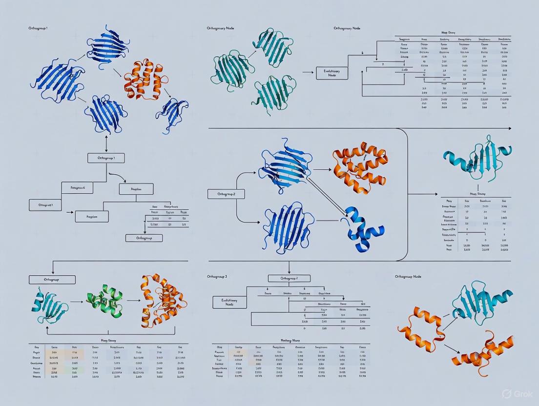
Visualizing Evolutionary Relationships and HOGs
The following diagrams illustrate the logical relationships between these concepts in an evolutionary tree and the corresponding data structure of a HOG.
Diagram 1: Evolutionary gene tree showing orthologs, paralogs, and co-orthologs. S1 and S2 are speciation events; D1 is a duplication event. Genes x1 and y1 are one-to-one orthologs. Genes x1 and x2 are in-paralogs with respect to S2. Genes x1 and y2 are out-paralogs with respect to S2. Genes x1 and x2 are co-orthologs with respect to z1 [14].
Diagram 2: Hierarchical structure of HOGs. A root HOG contains all descendants of an ancestral gene. At each taxonomic level (e.g., Vertebrate, Mammalian, Primate), the HOG is subdivided, reflecting duplications. At the primate level, a duplication event splits the mammalian HOG into two separate primate-level HOGs, B1 and B2 [15] [13].
Orthology Inference and HOG Construction in OMA
Protocol: OMA Orthology Inference Workflow
This protocol describes the step-by-step process used by the OMA algorithm to infer pairwise orthologs and construct HOGs [13].
Input Materials:
- Proteomes: Amino acid sequences for all species of interest in FASTA format.
- Species Tree: A phylogenetic tree representing the known evolutionary relationships among the input species.
Procedure:
- All-against-All Alignment: Perform a pairwise alignment of every protein in every proteome against every other protein to identify potential homologous sequences.
- Pairwise Ortholog Inference: For each pair of genomes, identify putative orthologs by filtering out out-paralogs while retaining in-paralogs. This step produces a list of pairwise orthologous relationships, each with a cardinality (1:1, 1:m, m:m) [15] [13].
- Construct Orthology Graph: Map the pairwise orthologs to a graph structure.
- Nodes: Represent individual genes.
- Edges: Represent inferred pairwise orthologous relationships between genes.
- Graph Cleaning: Identify and remove spurious edges (incorrect pairwise inferences) from the orthology graph to improve accuracy.
- Form Connected Components: Identify all connected components in the cleaned graph. Each connected component represents a putative gene family descended from a single ancestral gene.
- Build Hierarchical Orthologous Groups (HOGs):
- Traverse the species tree from the leaves (extant species) towards the root.
- At each taxonomic level (e.g., primates, mammals, vertebrates), group genes into a HOG if they descended from a single gene in the ancestor of that taxonomic level [15] [13].
- This results in a nested hierarchy of groups, where HOGs at recent clades are subsets of larger HOGs at older clades.
Outputs:
- A list of pairwise orthologs with relationship cardinalities.
- Hierarchical Orthologous Groups (HOGs) defined at various taxonomic levels.
- OMA Groups, which are cliques (fully connected subgraphs) of orthologs from the orthology graph [15].
Research Reagent Solutions for Orthology Inference
Table 2: Essential Materials and Tools for Orthogroup Analysis
| Resource/Tool | Type | Function in Analysis |
|---|---|---|
| OMA Browser [15] [13] | Database & Web Interface | Publicly accessible resource for querying pre-computed orthologs, HOGs, and OMA Groups across >2000 species. |
| FastOMA [11] | Software Algorithm | Scalable orthology inference tool for analyzing large-scale genomic datasets (thousands of genomes) with linear time complexity. |
| OMAmer [11] | Software Tool | Alignment-free tool for rapidly placing new protein sequences into pre-defined root HOGs using k-mers, used within the FastOMA pipeline. |
| NCBI Taxonomy [11] | Database | Reference taxonomy used by default in orthology inference to guide the species tree structure for HOG construction. |
| Species-specific Proteomes (e.g., from UniProt) | Data | Curated protein sequence sets for each species, serving as the primary input for the orthology inference pipeline. |
Application Notes for Evolutionary Analyses
Choosing the Right Type of Orthologs for Your Analysis
Different research questions require different types of orthology data. The table below guides selecting the appropriate data structure from OMA.
Table 3: Guide to Selecting Orthology Data Types in OMA
| Research Goal | Recommended Data Type | Rationale | Example Use Case |
|---|---|---|---|
| Genome Annotation Transfer | Pairwise Orthologs (1:1) | 1:1 orthologs show the highest degree of functional conservation, making them most reliable for transferring functional annotations between two specific species [13]. | Inferring the function of a newly sequenced mouse gene based on its 1:1 human ortholog. |
| Phylogenomic Profiling / Gene Presence-Absence | HOGs | HOGs provide a stable evolutionary unit across broad taxonomic ranges, allowing for consistent profiling of gene gains and losses in a lineage [13] [11]. | Profiling the evolutionary history of a gene family across eukaryotes to identify lineage-specific losses. |
| Analyzing Gene Duplication History | HOGs | The hierarchical structure of HOGs explicitly models duplication events at different taxonomic levels, making them ideal for studying the history of gene families [15] [13]. | Determining whether a duplication event in a gene family occurred before or after the radiation of mammals. |
| Species Tree Inference | OMA Groups | OMA Groups are cliques of orthologs where all members are mutually orthologous, minimizing the risk of including paralogs that could confound species tree reconstruction [15] [13]. | Constructing a robust species phylogeny using concatenated sequences of universal, single-copy orthologs. |
| Identifying Co-orthologs / In-paralogs | HOGs (at specific taxonomic levels) | HOGs defined at the level just after a duplication event will contain the co-orthologous copies. The in-paralogs are the genes within the same species in that HOG [14]. | Finding all human genes that are co-orthologous to a single Drosophila gene following a lineage-specific duplication in primates. |
Protocol: Identifying Co-orthologs and In-paralogs Using the OMA Browser
This protocol provides a practical method for researchers to find co-orthologs and in-paralogs for a gene of interest.
Objective: To identify all human co-orthologs and in-paralogs of a specific mouse gene using HOGs.
Procedure:
- Access the OMA Browser: Navigate to https://omabrowser.org [13].
- Search for Your Gene: In the search bar, enter the gene identifier (e.g., "TP53") or protein sequence and select the species of origin (e.g., Mus musculus) from the results.
- Navigate to the HOG View: On the gene page, locate and click the "Hierarchical Orthologous Groups" or "HOG" section/tab.
- Select the Relevant Taxonomic Level: The browser will display the HOGs containing your gene at different taxonomic levels. Identify the HOG defined at the last common ancestor of your species of interest. For example, to find human co-orthologs of a mouse gene, select the HOG at the "Euarchontoglires" or "Boreoeutheria" level, which is the common ancestor of mice and humans.
- Identify Co-orthologs and In-paralogs:
- Co-orthologs: All genes from the target species (e.g., human) within the selected HOG are co-orthologous to your query gene (e.g., mouse). If the mouse gene has in-paralogs, all human genes in the HOG are co-orthologous to all mouse genes in the HOG [14].
- In-paralogs: Within the HOG, all genes from the same species (e.g., multiple human genes) that resulted from a duplication after the speciation event defining the HOG are in-paralogs of each other [14].
Troubleshooting:
- No HOG found: The gene family might be species-specific or not conserved in the selected taxonomic scope. Try broadening the taxonomic level.
- Complex HOG structure: Multiple duplications can lead to complex HOGs. Carefully examine the HOG's taxonomic history to interpret relationships correctly.
The Orthology Conjecture represents a fundamental principle in comparative genomics, positing that orthologous genes—those related by vertical descent from a common ancestor through speciation—are more likely to conserve biological function than paralogous genes, which arise from gene duplication events [9]. This conjecture provides the foundational rationale for transferring functional annotations from characterized genes in model organisms to uncharacterized genes in newly sequenced genomes, driving discoveries across evolutionary biology, genetics, and drug development [9].
Despite its widespread application, the Orthology Conjecture has been subject to ongoing debate and empirical testing. A landmark study by Nehrt et al. challenged the conjecture, reporting that paralogs within the same species often exhibit greater functional similarity than orthologs between species at equivalent sequence divergence levels [16]. Subsequent research has contested these findings, with Altenhoff et al. demonstrating that after controlling for critical confounding factors—including authorship bias, variation in Gene Ontology term frequency, and propagated annotation bias—orthologs do indeed show weakly but significantly greater functional conservation than paralogs [17].
This Application Note provides a structured framework for assessing functional conservation between orthologous genes, offering standardized protocols and analytical resources designed for researchers investigating evolutionary relationships and functional genomics.
Quantitative Landscape of Functional Conservation
Comprehensive analysis of functional similarity between homologous genes requires careful consideration of multiple quantitative metrics derived from large-scale comparative studies. The table below summarizes key findings from major investigations testing the Orthology Conjecture.
Table 1: Comparative Functional Similarity Between Orthologs and Paralogs
| Study | Data Source | Ortholog Functional Similarity | Paralog Functional Similarity | Key Controlling Factors |
|---|---|---|---|---|
| Nehrt et al. (2011) [16] | 8,900 genes from human & mouse (Experimental GO) | BP: 0.4-0.5MF: 0.6-0.7 (no correlation with sequence identity) | Higher than orthologs at high sequence identities (≥70-80%) | Protein sequence identity |
| Altenhoff et al. (2012) [17] | 395,328 pairs from 13 genomes (Experimental GO) | Significantly higher than paralogs after bias correction | Significantly lower than orthologs after bias correction | Authorship bias, GO term frequency, background similarity, propagated annotation |
| Yeast-only analysis [17] | S. cerevisiae & S. pombe experimental annotations | Normalized functional similarity higher for orthologs | Normalized functional similarity lower for paralogs | Organism-specific annotation biases |
BP = Biological Process; MF = Molecular Function; GO = Gene Ontology
Critical confounding factors identified in these studies include:
- Authorship bias: Genes annotated in the same publication show inflated functional similarity [17]
- Propagated annotation bias: Computational function transfer artificially increases similarity among closely-related sequences [17]
- Background similarity variation: Intrinsic functional similarity differs across species pairs and biological contexts [17]
Table 2: Orthology Inference Tools and Benchmarking Metrics
| Method | Approach | Strengths | Orthobench Accuracy (F-score) |
|---|---|---|---|
| OrthoFinder [7] | Phylogenetic orthology inference with rooted gene trees | Most accurate ortholog inference; infers rooted species trees; comprehensive statistics | 3-24% higher than other methods [7] |
| PhylomeDB [7] | Tree-based database | Online resource with phylogenetic trees | Comparable to score-based methods |
| InParanoid [7] | Score-based heuristic | Fast pairwise ortholog identification | Lower than phylogenetic methods |
| OrthoMCL [18] | Graph-based clustering | Handles large datasets effectively | Lower than tree-based methods |
Experimental and Computational Protocols
Protocol 1: Phylogenetic Orthology Inference with OrthoFinder
Purpose: To identify orthologs and orthogroups across multiple species using phylogenetic methods.
Workflow:
Procedure:
Input Preparation
- Collect protein sequences in FASTA format for each species of interest
- Ensure consistent annotation and remove fragmented sequences
- For optimal results, include outgroup species to improve rooting accuracy
Software Execution
- Install OrthoFinder via conda:
conda install orthofinder -c bioconda - Run analysis:
orthofinder -f /path/to/protein/fasta/files/ - For large datasets, use
--assignoption to add species to existing analysis
- Install OrthoFinder via conda:
Result Interpretation
- Locate orthogroups in
Phylogenetic_Hierarchical_Orthogroups/N0.tsv - Find pairwise orthologs in
Orthologues/SpeciesX_vs_SpeciesY.tsv - Analyze gene duplication events in
Gene_Duplication_Events/
- Locate orthogroups in
Technical Notes: OrthoFinder's phylogenetic approach is 3-24% more accurate than heuristic methods on standard benchmarks [7]. The inclusion of outgroup species improves orthogroup inference accuracy by up to 20% [19].
Protocol 2: Controlled Functional Similarity Analysis
Purpose: To compare functional similarity between orthologs and paralogs while controlling for confounding biases.
Workflow:
Procedure:
Data Curation
- Obtain experimentally validated GO annotations (evidence codes EXP, IDA, IPI, IMP, IGI, IEP)
- Filter annotations to exclude those derived from common publications or authors
- Calculate species-specific GO term frequencies rather than using global frequencies
Similarity Measurement
- Use information-theoretic similarity measures that account for annotation specificity
- Calculate background similarity for random gene pairs within each species pair
- Normalize functional similarity scores against background similarity
Statistical Analysis
- Stratify comparisons by sequence identity bins (e.g., 50-60%, 60-70%, etc.)
- Use non-parametric tests (Mann-Whitney U) to compare orthologs vs. paralogs
- Perform sub-analysis focusing on specific functional categories (e.g., subcellular localization)
Technical Notes: This controlled approach revealed that orthologs show weakly but significantly higher functional similarity than paralogs, particularly for sub-cellular localization [17]. The effect is most pronounced when comparing orthologs between closely-related model organisms and human [17].
Research Reagent Solutions
Table 3: Essential Resources for Orthology and Functional Analysis
| Resource Category | Specific Tools/Databases | Primary Function | Application Context |
|---|---|---|---|
| Orthology Inference | OrthoFinder [7], OrthoMCL [18], OMA [18] | Identify orthologs and paralogs from sequence data | Evolutionary studies, functional annotation transfer |
| Functional Annotation | Gene Ontology (GO) database [17], Kyoto Encyclopedia of Genes and Genomes (KEGG) [20] | Standardized functional classification | Functional similarity quantification, pathway analysis |
| Benchmarking Resources | Orthobench [18], Quest for Orthologs [7] | Assess orthology inference accuracy | Method validation, tool selection |
| Sequence Databases | RefSeq [20], Pfam [20], eggNOG [20] | Protein families and domains reference | Gene family characterization, domain architecture analysis |
| Phylogenetic Analysis | IQ-TREE [18], MAFFT [18], TrimAL [18] | Multiple sequence alignment and tree inference | Gene tree estimation, evolutionary relationship resolution |
Concluding Remarks
The Orthology Conjecture remains a valuable guiding principle in comparative genomics, provided that analyses account for critical confounding factors and utilize robust phylogenetic methods. The protocols and resources presented here offer researchers a standardized framework for investigating functional conservation in evolutionary studies. As comparative genomics continues to expand—with recent discoveries of novel gene families from uncultivated taxa nearly tripling the known prokaryotic gene repertoire [20]—rigorous orthology assessment becomes increasingly essential for meaningful biological interpretation.
Orthology analysis forms the bedrock of comparative genomics, enabling researchers to trace the evolutionary history of genes across species. The conventional definition of orthology and paralogy is inherently genocentric, distinguishing genes related by speciation events (orthologs) from those related by duplication events (paralogs) [9]. This framework has guided functional annotation transfer for decades, operating on the principle that orthologs generally retain equivalent biological functions across different organisms [9].
However, several recent findings challenge this oversimplified perspective. Differences in domain architectures among proteins encoded by genes deemed orthologous are both common and functionally important, particularly in multicellular eukaryotes [9]. The pervasive nature of alternative splicing and alternative transcription further complicates genocentric definitions [9]. These realities necessitate a conceptual shift toward smaller, more stable evolutionary units—specifically protein domains and even sub-gene elements—to accurately describe evolutionary processes and functional relationships [9].
This Application Note details methodologies for identifying and analyzing these finer-grained evolutionary units, providing practical frameworks for researchers investigating gene evolution, function, and innovation.
Theoretical Framework: From Genes to Evolutionary Units
The Hierarchical Nature of Orthology
Orthologous relationships extend beyond simple one-to-one correspondences between genes. Complex evolutionary scenarios involving lineage-specific duplications and losses create intricate relationships best described through hierarchical orthologous groups (HOGs) [11]. HOGs represent sets of genes that descended from a single ancestral gene at each speciation node in a species tree, creating a nested structure that mirrors evolutionary history [11].
Table 1: Key Concepts in Modern Orthology Analysis
| Concept | Definition | Evolutionary Significance |
|---|---|---|
| Orthologs | Genes related by speciation events [9] | Trace species divergence; often retain core biological functions |
| Paralogs | Genes related by duplication events [9] | Enable functional innovation through duplication and divergence |
| Hierarchical Orthologous Groups (HOGs) | Sets of genes descending from a single ancestral gene at specific tree levels [11] | Capture nested evolutionary relationships across taxonomic levels |
| Root HOG | Coarse-grained gene family originating from ancestral gene at analysis root [11] | Provides framework for large-scale orthology inference |
| In-paralogs | Paralogs that duplicated after a given speciation event [9] | Indicate lineage-specific gene family expansions |
Limitations of Genocentric Orthology
The genocentric orthology model faces several critical limitations that impact evolutionary analysis and functional inference. Between-species differences in domain architectures of homologous proteins create complex networks of relationships that cannot be properly represented under genocentric definitions [9]. When proteins contain repetitive, promiscuous domains—such as ankyrin repeats or tetratricopeptide repeats—the concept of orthology at the gene level essentially breaks down [9].
These limitations have driven the recognition that stable evolutionary units often exist below the gene level. The correct description of evolutionary processes may ultimately require tracing the fates of individual nucleotides or stable protein domains, moving beyond genocentric orthology to a more nuanced framework [9].
Diagram 1: Genocentric vs. domain-centric evolutionary views (47 characters)
Methodological Approaches and Tools
Scalable Orthology Inference with FastOMA
The FastOMA algorithm addresses critical scalability challenges in orthology inference, enabling processing of thousands of eukaryotic genomes within 24 hours while maintaining high accuracy [11]. This linear scalability represents a significant advancement over traditional methods with quadratic time complexity, such as OrthoFinder and SonicParanoid [11].
FastOMA employs a two-step methodology for efficient orthology inference. First, it maps input proteomes onto reference HOGs using the alignment-free OMAmer tool, which uses k-mer-based placement for coarse-grained family assignment [11]. Subsequently, it resolves the nested structure of HOGs through leaf-to-root traversal of the species tree, identifying genes grouped together at each taxonomic level [11].
Table 2: Performance Benchmarks of Orthology Inference Tools
| Method | Time Complexity | Reference Proteomes Processed in 24 Hours | Precision (SwissTree) | Recall (SwissTree) |
|---|---|---|---|---|
| FastOMA | Linear [11] | 2,086 [11] | 0.955 [11] | 0.69 [11] |
| OMA | Quadratic [11] | ~50 [11] | ~0.94* | ~0.65* |
| OrthoFinder | Quadratic [11] | Not specified | High recall [11] | Highest [11] |
| SonicParanoid | Quadratic [11] | Not specified | Moderate | Moderate |
Table 3: FastOMA Algorithmic Steps and Applications
| Step | Process | Tools Used | Output |
|---|---|---|---|
| Gene Family Inference | Map proteomes to reference HOGs | OMAmer [11] | Query rootHOGs |
| Unplaced Sequence Handling | Cluster unmapped sequences | Linclust [11] | Additional rootHOGs |
| Orthology Inference | Resolve nested HOG structure | Tree traversal [11] | Hierarchical Orthologous Groups |
| Downstream Analysis | Evolutionary interpretation | OMA ecosystem [11] | Phylogenetic profiles, gene histories |
Specialized Tools for Domain-Centric Analysis
AlgaeOrtho provides a specialized framework for processing ortholog inference results with a user-friendly interface [21]. Built upon SonicParanoid and the PhycoCosm database, it generates ortholog tables, similarity heatmaps, and unrooted protein trees to visualize putative orthologs across algal species [21]. This tool is particularly valuable for identifying bioengineering targets in non-model organisms, as it doesn't depend on existing protein annotations [21].
For basic ortholog identification, BLAST remains a fundamental tool. The BLASTP algorithm searches protein sequences against protein databases, with results filtered by metrics including query coverage, percent identity, and E-value (statistical measure of match significance) [22]. This approach enables ortholog discovery even in species without well-annotated genomes [22].
Diagram 2: FastOMA orthology inference workflow (42 characters)
Experimental Protocols
Protocol: Domain-Centric Orthology Analysis
Objective: Identify orthologous domains and sub-gene elements across multiple species, moving beyond genocentric definitions.
Materials and Reagents:
- Multi-species proteome datasets in FASTA format
- High-performance computing cluster (300+ CPU cores for large-scale analyses)
- FastOMA software suite (https://github.com/DessimozLab/FastOMA/)
- AlgaeOrtho tool for specialized taxonomic groups
- BLAST+ suite for sequence similarity searches
- Reference taxonomic tree (NCBI taxonomy or TimeTree resource)
Procedure:
Data Preparation and Quality Control
- Download proteome datasets from PhycoCosm, UniProt, or organism-specific databases
- Validate file formats and sequence integrity
- For fragmented gene models, enable FastOMA's handling of fragmented sequences [11]
FastOMA Execution and Parameter Optimization
Domain-Centric Orthology Resolution
- Extract domain architecture information from HOG members using domain databases
- Identify orthologous relationships at the domain level rather than gene level
- Analyze domain gain/loss events across the phylogenetic tree
Validation and Visualization
Troubleshooting:
- Low orthology resolution may indicate overly stringent OMAmer thresholds
- Excessive splitting of gene families may require adjustment of rootHOG merging parameters
- For non-model organisms with limited annotation, use AlgaeOrtho's annotation-independent approach [21]
Protocol: Sub-gene Element Identification
Objective: Identify and trace the evolutionary history of sub-gene elements, including specific protein domains and repetitive elements.
Materials and Reagents:
- Protein sequences with domain annotation
- Domain database (Pfam, InterPro)
- Multiple sequence alignment tools (Clustal Omega, MAFFT)
- Custom scripts for domain boundary extraction
Procedure:
Domain Annotation and Extraction
- Annotate protein sequences using domain databases
- Extract individual domain sequences based on annotated boundaries
- Create domain-specific sequence datasets for orthology analysis
Domain-Centric Orthology Inference
- Process domain sequences through standard orthology inference pipelines
- Compare domain-level orthology assignments with gene-level assignments
- Identify instances where domain orthology contradicts gene orthology
Evolutionary Analysis of Sub-gene Elements
- Reconstruct phylogenetic trees for individual domains
- Compare domain trees with species trees to identify horizontal transfer events
- Analyze evolutionary rates of domains versus full-length proteins
The Scientist's Toolkit: Research Reagent Solutions
Table 4: Essential Research Reagents and Resources for Evolutionary Analysis
| Resource | Type | Primary Function | Application Context |
|---|---|---|---|
| FastOMA | Software Algorithm | Large-scale orthology inference [11] | Genome-wide ortholog identification across thousands of species |
| OMAmer | Software Tool | k-mer-based sequence placement [11] | Ultrafast homology clustering and gene family assignment |
| AlgaeOrtho | Web Application | Ortholog visualization [21] | User-friendly ortholog identification in algal species |
| PhycoCosm | Database | Multi-omics data for algae [21] | Source of annotated proteomes for non-model organisms |
| BLAST+ Suite | Software Tools | Sequence similarity search [22] | Initial ortholog candidate identification and validation |
| TimeTree | Database | Species divergence times [11] | High-resolution species trees for improved orthology inference |
| Linclust | Software Algorithm | Sequence clustering [11] | Grouping unmapped sequences into rootHOGs |
| Tri-O-acetyl-D-glucal | Tri-O-acetyl-D-glucal, CAS:2873-29-2, MF:C12H16O7, MW:272.25 g/mol | Chemical Reagent | Bench Chemicals |
| 5-Hydroxythiabendazole | 5-Hydroxythiabendazole | High-Purity Reference Standard | 5-Hydroxythiabendazole: A key metabolite for thiabendazole research. For Research Use Only. Not for human or veterinary diagnostic or therapeutic use. | Bench Chemicals |
The move beyond genocentric definitions to domains and sub-gene elements represents a fundamental shift in evolutionary analysis. This approach acknowledges the complexity of gene evolution and provides a more accurate framework for understanding functional relationships across species. The protocols and tools outlined in this Application Note empower researchers to implement this refined evolutionary perspective in their orthogroup analyses.
Future methodological developments will likely focus on integrating structural protein data to improve resolution at deeper evolutionary levels, as well as incorporating gene order conservation as additional evidence for orthology assessment [11]. As sequencing initiatives continue to expand genomic datasets, these domain-centric approaches will become increasingly essential for extracting meaningful biological insights from the deluge of sequence data.
Conducting Orthogroup Analysis: A Step-by-Step Protocol from Sequence to Biological Insight
In comparative genomics, accurately identifying homology relationships between genes is fundamental to understanding evolutionary history, gene function, and phenotypic diversity. Orthologs, genes originating from speciation events, are particularly crucial for transferring functional annotations across species and reconstructing evolutionary relationships. The challenge of orthology inference has spawned two predominant computational approaches: phylogenetic tree-based methods and graph-based clustering methods. Tree-based methods like OrthoFinder leverage phylogenetic analyses to delineate evolutionary relationships, while graph-based approaches like SonicParanoid and Broccoli utilize sequence similarity networks and clustering algorithms. For researchers conducting orthogroup analysis in evolutionary studies, selecting the appropriate tool requires understanding their fundamental methodologies, performance characteristics, and suitability for specific biological questions. This Application Note provides a structured comparison of these prominent orthology inference algorithms to guide researchers in selecting optimal tools for their genomic investigations.
Algorithmic Foundations and Methodological Comparisons
Core Principles and Technical Implementations
OrthoFinder employs a comprehensive phylogenetic methodology that extends beyond basic orthogroup inference. The algorithm begins with all-versus-all sequence similarity searches but incorporates a critical innovation: a novel score transformation that eliminates gene length bias in orthogroup detection. This transformation normalizes BLAST scores based on sequence length, preventing the systematic under-clustering of short genes and over-clustering of long genes that plagued earlier methods [3]. Following this normalization, OrthoFinder infers gene trees for all orthogroups, reconstructs a rooted species tree, and maps gene duplication events to both gene and species trees [7]. This phylogenetic approach allows OrthoFinder to provide rooted gene trees, ortholog identification, and gene duplication events mapped to specific branches in the species tree. The algorithm can utilize either fast similarity search tools like DIAMOND or more accurate multiple sequence alignment and phylogenetic inference methods based on user preference [7].
SonicParanoid2 represents a substantial update to the original graph-based algorithm, incorporating machine learning to enhance performance. The methodology employs two key innovations: an AdaBoost classifier that predicts and executes faster alignment directions between proteome pairs, thereby avoiding unnecessary computations, and a Doc2Vec language model that enables domain-aware orthology inference for proteins with complex domain architectures [23]. The algorithm first performs graph-based orthology inference using the optimized alignments, then conducts separate domain-based orthology inference, and finally merges the results before applying the Markov Cluster Algorithm (MCL) to infer multi-species orthogroups [23]. This hybrid approach allows SonicParanoid2 to maintain high speed while improving recall for difficult-to-detect orthologs in duplication-rich genomes.
Broccoli employs a distinct graph-based approach that reduces computational burden through k-mer clustering rather than all-versus-all alignments. The method builds similarity networks using reciprocal smallest distance pairs and applies clustering to identify homologous families. Unlike simpler graph methods, Broccoli incorporates phylogenetic information by building multiple sequence alignments and distance trees to refine orthogroup predictions [24]. This combination of fast similarity filtering with subsequent phylogenetic refinement enables Broccoli to achieve a balance between speed and accuracy, particularly for larger datasets.
Workflow Comparison and Logical Relationships
The following diagram illustrates the core methodological differences and relationships between the phylogenetic and graph-based approaches to orthology inference:
Figure 1: Workflow comparison between phylogenetic and graph-based orthology inference approaches, highlighting core methodological differences.
Performance Benchmarking and Comparative Analysis
Quantitative Performance Metrics
Empirical evaluations across diverse datasets provide critical insights into the practical performance characteristics of orthology inference tools. The following table summarizes key benchmark results from standardized assessments:
Table 1: Performance comparison of orthology inference tools on standardized benchmark datasets
| Tool | Approach | Execution Time (QfO dataset) | Memory Footprint | Orthobench Accuracy (F-score) | Scalability (2000 MAGs) |
|---|---|---|---|---|---|
| OrthoFinder | Phylogenetic | 1x (reference) | Moderate | Highest [7] | Failed to complete [23] |
| SonicParanoid2 | Graph-based + ML | 0.28x (fast mode) to 0.83x (default) | Moderate | Most accurate in recent benchmarks [23] | 1.7 days (default mode) [23] |
| Broccoli | Graph-based + phylogenetic refinement | 0.4x (fast mode) | Highest | High [24] | Failed to complete [23] |
| ProteinOrtho | Graph-based with heuristics | 0.8x (similar settings) | Lowest | Not reported | 5.7 days [23] |
Biological Context Performance
Different biological contexts present unique challenges for orthology inference. A study evaluating performance across Brassicaceae species with varying ploidy levels revealed important practical considerations:
Table 2: Algorithm performance across biological contexts with different genomic complexities
| Tool | Diploid Species Sets | Mixed Ploidy Species Sets | Notes on Biological Accuracy |
|---|---|---|---|
| OrthoFinder | High accuracy, well-resolved groups | Maintains accuracy with complex histories | Better handling of duplication events [24] |
| SonicParanoid | High consistency with other methods | Good performance with ploidy variation | Slight discrepancies in gene content [24] [25] |
| Broccoli | Similar results to OrthoFinder/SonicParanoid | Effective with complex gene histories | Useful for initial predictions [24] |
| OrthNet | Outlier results in comparisons | Provides synteny information | Useful for colinearity analysis [24] |
Application to specific biological questions further illuminates performance differences. In identifying cold-responsive transcription factors across eudicots, orthogroup analysis successfully identified 35 high-confidence conserved cold-responsive transcription factor orthogroups (CoCoFos), including both well-characterized regulators and novel candidates [26]. This demonstrates the practical utility of these methods for discovering functionally relevant gene families across species.
Experimental Protocols and Implementation Guidelines
Standard Orthology Inference Protocol
Materials and Input Requirements
- Protein sequence files: One FASTA file per species with amino acid sequences
- Computational resources: Multi-core processor, sufficient RAM (≥16GB recommended), storage space
- Software dependencies: Python 3.6+, BioPython, NumPy, SciPy (for OrthoFinder); additional aligners optional
Procedure
- Data Preparation
- Download or assemble proteomes for all species of interest
- Ensure consistent annotation quality across species
- Format as individual FASTA files with appropriate identifiers
Tool Installation
Basic Execution
Result Interpretation
- OrthoFinder: Analyze Orthogroups/Orthogroups.tsv and PhylogeneticHierarchicalOrthogroups/N0.tsv
- SonicParanoid2: Examine ortholog clusters in output directory
- Broccoli: Review final_orthogroups.txt and phylogenetic trees
Decision Framework for Tool Selection
The following diagram provides a structured approach for selecting the most appropriate orthology inference tool based on research objectives and dataset characteristics:
Figure 2: Decision framework for selecting orthology inference tools based on research goals and practical constraints.
Table 3: Essential research reagents and computational resources for orthology inference studies
| Resource Category | Specific Tools/Resources | Function/Purpose | Availability |
|---|---|---|---|
| Core Inference Algorithms | OrthoFinder, SonicParanoid2, Broccoli | Primary orthogroup inference | GitHub, Bioconda, GitLab |
| Sequence Search Tools | DIAMOND, MMseqs2, BLAST | Accelerated similarity searches | Standalone packages |
| Multiple Sequence Alignment | MAFFT, MUSCLE, Clustal Omega | Alignment for phylogenetic methods | Package managers |
| Phylogenetic Inference | IQ-TREE, RAxML, FastTree | Gene tree reconstruction | Package managers |
| Benchmarking Resources | OrthoBench, Quest for Orthologs | Method validation and comparison | Online platforms |
| Specialized Databases | OMA, OrthoDB, EggNOG | Reference orthogroups and functional annotations | Web access, downloads |
| Visualization Tools | ITOL, FigTree, Cytoscape | Results exploration and presentation | Web-based, standalone |
Orthology inference remains a cornerstone of comparative genomics and evolutionary studies, with method selection significantly impacting downstream analyses. Based on current benchmarking results and methodological considerations:
For comprehensive evolutionary analyses requiring gene trees, duplication event mapping, and species tree inference, OrthoFinder provides the most complete phylogenetic framework, particularly for datasets where computational resources are not limiting [7].
For large-scale analyses or projects prioritizing computational efficiency, SonicParanoid2 offers an optimal balance of speed and accuracy, with machine learning enhancements that improve performance on complex gene families [23].
For standard orthogroup identification with phylogenetic refinement, Broccoli represents a viable middle ground, though scalability limitations may affect very large datasets [24].
Validation with biological benchmarks remains essential, as different methods may perform variably across specific taxonomic groups or gene families of interest [24] [18].
Future methodological developments will likely continue blending phylogenetic rigor with computational efficiency, further narrowing the performance gaps between approaches. Researchers should consider starting with rapid graph-based methods for initial exploration followed by more comprehensive phylogenetic analyses for specific gene families of interest, thereby leveraging the complementary strengths of both approaches in orthogroup analysis for evolutionary studies.
High-quality proteome data is foundational for accurate orthogroup analysis in evolutionary studies. The identification of orthologous genes—genes diverged after a speciation event—relies on precise inference from protein sequences [9]. OrthoFinder, a leading phylogenetic orthology inference method, uses protein sequences as its primary input to infer orthogroups, gene trees, and ultimately the rooted species tree [7]. The quality of input proteomes directly impacts the accuracy of distinguishing orthologues from paralogues, which is crucial for understanding gene function evolution and reconstructing species relationships [9]. This protocol outlines best practices for acquiring and pre-processing proteomic data to ensure reliable downstream orthogroup analysis.
Proteome Acquisition Strategies and Experimental Design
The method of proteome acquisition determines the type of input data available for orthogroup analysis. The choice between bottom-up and top-down approaches significantly impacts the protein sequences that will form the basis of orthology inference.
Table 1: Mass Spectrometry Acquisition Methods for Proteomics
| Method Type | Description | Best For | Key Considerations |
|---|---|---|---|
| Data-Dependent Acquisition (DDA) | Selects most abundant precursors for fragmentation | Discovery proteomics, hypothesis generation | Risk of undersampling low-abundance species; requires spectral libraries [27] |
| Data-Independent Acquisition (DIA) | Fragments all precursors in predefined m/z windows | Large-scale studies, enhanced reproducibility | Enables retrospective analysis; improved with AI-driven tools like DIA-NN [27] |
| Selected Reaction Monitoring (SRM)/Multiple Reaction Monitoring (MRM) | Monitors specific predefined precursors | Targeted proteomics, absolute quantitation | High sensitivity; uses heavy isotope-labeled internal standards [27] |
For evolutionary studies where the goal is comprehensive proteome coverage for orthogroup inference, DIA methods are increasingly favored due to their comprehensive sampling of detectable peptides. Advances in hybrid MS systems such as Orbitrap Astral and timsTOF have dramatically improved sensitivity, dynamic range, and proteome coverage [27] [28]. For single-cell proteomics, which can provide insights into cellular heterogeneity in evolutionary contexts, the choice between DDA with tandem mass tags (TMT) and DIA with label-free quantification involves trade-offs between throughput and quantitative accuracy [28].
Special Considerations for Non-Model Organisms
For non-model organisms lacking well-annotated genomes, Proteomics Informed by Transcriptomics (PIT) approaches can generate sample-specific protein databases from RNA-seq data [29]. The Galaxy Integrated Omics (GIO) platform provides standardized workflows for PIT analysis, including:
- PIT protein identification without a reference genome
- PIT protein identification using a genome guide
- PIT genome annotation [29]
These approaches are particularly valuable for evolutionary studies of non-model organisms where reference proteomes are unavailable or incomplete.
Pre-processing Workflow: From Raw Data to Protein Identification
The conversion of raw MS data into reliable protein identifications requires rigorous preprocessing to manage technical variability and ensure data quality. Adherence to standardized workflows is essential for generating comparable datasets for cross-species orthogroup analysis.
Diagram 1: Proteomics Data Pre-processing Workflow for Orthogroup Analysis
Data Standardization and Peak Detection
The initial preprocessing step involves converting vendor-specific raw data files (.RAW for Thermo, .d for Bruker/Agilent, .WIFF for Sciex) to standardized open formats (mzML, mzXML) using tools like MSConvert from ProteoWizard [27]. This ensures compatibility with open-source preprocessing software and facilitates data sharing for collaborative evolutionary studies. Subsequent peak detection and feature extraction algorithms identify peptide features from the raw spectra, followed by retention time alignment across samples to correct for experimental variations [27].
Protein Identification and Quality Control
Peptide-spectrum matching (PSM) compares experimental spectra against theoretical databases, which can include reference proteomes or sample-specific databases generated via PIT approaches [29] [27]. To ensure reliability for orthogroup analysis, strict false discovery rate (FDR) control is essential. According to Human Proteome Organization (HUPO) 2023 guidelines:
- Each protein identification must be supported by at least two distinct, non-nested peptides of nine or more amino acids in length
- Global FDR must be controlled at ≤1% for both peptide-spectrum matches and protein identifications [27]
Table 2: Software Tools for Proteomics Data Pre-processing
| Software | Acquisition Type | Primary Use | Strengths |
|---|---|---|---|
| MaxQuant | DDA | Discovery proteomics | Comprehensive workflow; label-free and label-based quantitation [27] |
| FragPipe | DDA | Discovery proteomics | Integrated platform; uses MSFragger for fast searching [27] |
| DIA-NN | DIA | Discovery proteomics | Library-free analysis; AI-predicted spectra; high reproducibility [27] |
| Spectronaut | DIA | Discovery proteomics | Professional solution; strong performance with spectral libraries [27] |
| PEAKS | DDA/DIA | De novo sequencing | Critical for non-model organisms without reference genomes [27] |
| Skyline | Targeted | Absolute quantitation | Method development for SRM/PRM; uses heavy isotope standards [27] |
For single-cell proteomics, which can reveal evolutionary differences at cellular resolution, specialized computational workflows address pervasive missing data challenges through normalization and imputation techniques [28]. The choice between DIA-LFQ and DDA-TMT involves trade-offs: DDA-TMT enables multiplexing (up to 35 channels) but suffers from ratio compression, while DIA-LFQ provides more accurate quantification but typically requires separate runs for each cell [28].
Quantitative Strategies and Data Quality Assessment
Quantitative proteomics provides valuable evolutionary insights, particularly for studying gene expression divergence. The choice of quantitative method depends on the evolutionary questions being addressed and the sample types available.
Label-Free vs. Label-Based Quantitation
Label-free quantitation (LFQ) methods directly compare peptide intensities across samples, making them suitable for large-scale evolutionary studies with many samples [27]. Common LFQ approaches include:
- Intensity-based absolute quantitation (iBAQ): normalizes peptide intensities by protein length
- Spectral counting: counts PSMs corresponding to each protein
- LFQ intensity: uses the MaxLFQ algorithm for accurate label-free quantification
Label-based quantitation uses chemical (TMT, iTRAQ) or metabolic (SILAC) labeling to incorporate stable isotopes, enabling multiplexed comparisons within a single experiment [27]. While offering enhanced precision and throughput, label-based methods are limited by available labeling channels and may experience ratio compression effects.
Quality Control and Normalization
Post-quantitation, protein abundances undergo log2 transformation and normalization (e.g., total ion current or median normalization) to improve data distribution [27]. Missing values are imputed using methods such as k-nearest neighbors (kNN) or random forest, though careful evaluation is required to avoid artifactual changes. Statistical tools like Limma and MSstats facilitate differential expression analysis, while interactive platforms (Prodigy, SpectroPipeR) generate integrated reports with PCA, heatmaps, and clustering to identify outliers or batch effects [27].
Orthology Inference from Processed Proteomes
With quality-controlled proteome data, orthology inference can proceed using phylogenetic methods. OrthoFinder provides comprehensive analysis by integrating multiple steps: orthogroup inference, gene tree inference, rooted species tree inference, and gene duplication event identification [7].
Diagram 2: Orthology Inference Workflow from Processed Proteomes
OrthoFinder uses sequence similarity searches (default: DIAMOND) as raw data for orthogroup inference and gene tree inference using DendroBLAST [7]. The method has demonstrated superior accuracy, outperforming other methods by 3-24% on SwissTree and 2-30% on TreeFam-A benchmarks in the Quest for Orthologs assessment [7]. This high accuracy is crucial for reliable evolutionary interpretations, as orthologous genes are generally assumed to retain equivalent functions in different organisms, though this orthology-function conjecture has nuances and exceptions [9].
Research Reagent Solutions for Proteome Acquisition
Table 3: Essential Research Reagents and Platforms for Proteomics
| Category | Specific Tools/Platforms | Function in Proteome Acquisition |
|---|---|---|
| LC-MS Systems | Orbitrap Astral MS, timsTOF MS | High-sensitivity mass spectrometry for comprehensive proteome coverage [27] [28] |
| Sample Preparation | cellenONE, Evosep One tips, proteoCHIP | Automated, low-volume sample processing minimizing protein loss [28] |
| Multiplexing Reagents | TMT (Tandem Mass Tags), iTRAQ | Chemical labeling for multiplexed analysis of multiple samples [27] [28] |
| Separation Columns | μPAC (micro-pillar array columns) | Specialized columns for single-cell proteomics applications [28] |
| Database Search | MS-GF+, SearchGUI | Peptide spectrum matching against protein databases [29] [27] |
| Internal Standards | Heavy isotope-labeled peptides | Absolute quantitation in targeted proteomics [27] |
Experimental Protocol: Standard Proteomics Workflow for Orthogroup Analysis
Sample Preparation and MS Acquisition
- Cell Lysis and Protein Extraction: Use appropriate lysis buffers compatible with downstream processing. For single-cell protocols, consider one-pot approaches that omit reduction and alkylation to minimize sample loss [28].
- Protein Digestion: Digest proteins with trypsin (typically in a 1:50 enzyme-to-protein ratio) at 37°C for 12-16 hours. For single-cell proteomics, adding trypsin in two boluses rather than a single addition improves digestion efficiency [28].
- Peptide Cleanup: Desalt peptides using C18 solid-phase extraction tips or columns.
- LC-MS/MS Analysis: Separate peptides using nanoflow liquid chromatography (typically C18 columns) with gradient elution (typically 60-120 minutes). Acquire data using DIA methods for comprehensive coverage or DDA for library generation.
Data Processing and Protein Identification
- Convert Raw Files: Use MSConvert (ProteoWizard) to transform vendor-specific files to mzML format [27].
- Database Search: Use appropriate software (Table 2) with the following parameters:
- Precursor mass tolerance: 10-20 ppm
- Fragment mass tolerance: 0.02-0.05 Da
- Enzyme specificity: trypsin with up to 2 missed cleavages
- Fixed modifications: carbamidomethylation of cysteine
- Variable modifications: oxidation of methionine, protein N-terminal acetylation
- FDR Control: Apply 1% FDR at both peptide and protein levels using target-decoy approaches [27].
- Protein Assembly: Apply parsimony principles to assign peptides to minimal number of proteins.
Data Export for Orthology Analysis
Export identified proteins in FASTA format containing all protein sequences detected across samples/species. Ensure consistent header formatting with unique identifiers and source organism information. For OrthoFinder analysis, provide one FASTA file per species.
Robust proteome acquisition and preprocessing are critical for reliable orthogroup analysis in evolutionary studies. By following standardized workflows, implementing rigorous quality control, and selecting appropriate quantitative strategies, researchers can generate high-quality proteomic data that enables accurate inference of orthologous relationships. The integration of advanced mass spectrometry platforms with sophisticated computational tools like OrthoFinder provides a powerful framework for evolutionary genomics, allowing researchers to reconstruct gene family evolution and species relationships with increasing accuracy and comprehensiveness.
OrthoFinder is a powerful platform for phylogenetic orthology inference, enabling researchers to determine evolutionary relationships between genes across multiple species. For evolutionary studies, identifying orthogroups—sets of genes descended from a single gene in the last common ancestor of the species considered—is a fundamental step. Unlike heuristic methods that rely solely on sequence similarity, OrthoFinder provides a comprehensive phylogenetic analysis, inferring orthogroups and orthologs, reconstructing rooted gene trees, identifying all gene duplication events, and inferring a rooted species tree [30]. This protocol guides you through a complete OrthoFinder analysis, from data preparation to interpretation of results, framed within the context of orthogroup analysis for evolutionary research.
OrthoFinder Algorithm and Theoretical Framework
Core Algorithmic Steps
The OrthoFinder algorithm transforms protein sequences into a complete phylogenetic analysis through several integrated steps [30]:
- Orthogroup Inference: Groups homologous genes into orthogroups using sequence similarity data.
- Gene Tree Inference: Infers a gene tree for each orthogroup.
- Species Tree Inference: Analyzes gene trees to infer a rooted species tree.
- Gene Tree Rooting: Roots all gene trees using the inferred species tree.
- Duplication-Loss-Coalescence Analysis: Analyzes rooted gene trees to identify orthologs, paralogs, and gene duplication events, mapping them to both gene trees and the species tree.
Advantages of Phylogenetic Orthology Inference
OrthoFinder's phylogenetic approach provides significant advantages over similarity-score-based methods. While heuristic methods are confounded by variable sequence evolution rates, phylogenetic trees can distinguish between variable evolution rates (branch lengths) and divergence order (tree topology), leading to more accurate identification of orthology and paralogy relationships [30]. Benchmark tests have demonstrated that OrthoFinder achieves 3–24% higher accuracy in ortholog inference compared to other methods [30].
Experimental Design and Planning
Defining the Research Objective
Your experimental design should align with one of three common comparative genomics approaches:
Table: OrthoFinder Experimental Design Strategies
| Research Objective | Species Selection Strategy | Key Considerations |
|---|---|---|
| Clade Comparison | Include all available species within the clade of interest | Usually no need for an outgroup; improves orthogroup resolution [31] |
| Ortholog Identification | Include 6-10 species to break up long branches [31] | Absolute minimum of 4 species; prevents inaccurate inference [31] |
| Specific Evolutionary Event | Target species around the branch of interest | Include ≥2 species below, ≥2 on closest branch above, and ≥2 outgroup species [31] |
Species and Data Selection
Select high-quality annotated genomes whenever possible. OrthoFinder is reasonably robust to missing genes, but transcriptome data with ~100,000 transcripts per species can be computationally challenging [31]. For evolutionary studies, including appropriately sampled species is crucial for breaking up long branches in the species tree, which significantly improves orthology assignment accuracy [32].
Materials and Reagents
Research Reagent Solutions
Table: Essential Materials for OrthoFinder Analysis
| Item | Specification/Function | Source Examples |
|---|---|---|
| Species Proteomes | Amino acid sequences in FASTA format; one file per species | Ensembl, Phytozome, JGI [33] [31] |
| Computing Resources | Multi-core processor, sufficient RAM, disk space | Computer cluster recommended for large analyses (>50 species) |
| Software Dependencies | Python, NumPy, SciPy; bundled in standalone version | Bioconda (conda install orthofinder -c bioconda) [19] |
| Sequence Search Tool | DIAMOND (default) or BLAST for similarity searches | OrthoFinder uses DIAMOND by default for speed [30] |
Step-by-Step Protocol
Data Acquisition and Preparation
Downloading Proteomes
- Create a dedicated working directory without spaces in the path (e.g.,
~/orthofinder_analysis/proteomes/) [33]. - Obtain proteomes from reliable sources such as Ensembl:
- Navigate to https://www.ensembl.org/
- Select your species of interest
- Under "Gene annotation," click "Download FASTA"
- Access the "pep" folder and download the "
.pep.all.fa.gz" file [33]
- Repeat for all species in your analysis.
Proteome Preprocessing
- Decompress downloaded files:
- Extract primary transcripts (critical step): This step reduces runtime and improves accuracy by selecting the longest transcript per gene [33].
- Rename files to concise, identifiable names (e.g.,
Homo_sapiens.fa). OrthoFinder uses filenames as species identifiers in results [31].
OrthoFinder Execution
Basic Command
Run OrthoFinder on the prepared proteomes:
The analysis time varies from 20 minutes to several hours depending on the number of species, genes, and computer processing cores [33].
Workflow Diagram
Results Interpretation and Analysis
Initial Quality Assessment
After OrthoFinder completes, check the summary statistics in the terminal output or in Comparative_Genomics_Statistics/Statistics_Overall.tsv [32]. Key metrics include:
- Percentage of genes assigned to orthogroups: >80% is generally acceptable; <80% may indicate poor species sampling [32]
- Number of orthogroups
- Orthogroup size statistics (G50 and O50)
Examine Comparative_Genomics_Statistics/Statistics_PerSpecies.tsv to identify species with low assignment rates, which may have long branches in the species tree due to insufficient sampling of closely related species [32].
Analyzing the Species Tree
The rooted species tree is found in Species_Tree/SpeciesTree_rooted.txt [32].
- OrthoFinder automatically roots the tree using the STRIDE algorithm [32]
- Verify the tree topology matches expected species relationships
- Long branches indicate poor species sampling; consider adding intermediate species to improve future analyses [32]
- Support values are derived from the proportion of single-locus gene trees supporting each bipartition (STAG algorithm), which is more stringent than standard bootstrap support [32]
Identifying Orthologs of Interest
To find orthologs for a specific gene:
- Navigate to the
Orthologues/directory - Open the species-specific subdirectory (e.g.,
Orthologues_Drosophila_melanogaster/) - Locate the relevant pairwise comparison file (e.g.,
Drosophila_melanogaster__v__Homo_sapiens.tsv) - Find your gene of interest in the table, which provides:
- Orthogroup identifier
- Orthologous genes in the target species [32]
Investigating Gene Trees and Duplication Events
Gene trees provide evolutionary context for orthology relationships:
- Trees are located in
Gene_Trees/(without support values) orResolved_Gene_Trees/(with node labels for duplication events) [32] - OrthoFinder automatically roots gene trees, making interpretation straightforward [32]
- Complex orthology relationships (e.g., one-to-many) often result from gene duplication events [32]
To investigate gene duplication events in a specific clade:
- Open
Species_Tree/SpeciesTree_rooted_node_labels.txtto identify node labels - Check
Gene_Duplication_Events/Duplications.tsvfor events at specific nodes - Cross-reference with orthogroups of interest to understand duplication history [32]
Advanced Applications in Evolutionary Research
Hierarchical Orthogroups for Specific Clades
For evolutionary studies focusing on specific clades, OrthoFinder's hierarchical orthogroups (HOGs) are particularly valuable:
- HOGs are defined at each node of the species tree, providing orthogroups for specific clades [19]
- Located in
Phylogenetic_Hierarchical_Orthogroups/asN0.tsv,N1.tsv, etc., corresponding to nodes in the species tree [19] - According to OrthoBench benchmarks, these phylogenetically-informed orthogroups are 12-20% more accurate than graph-based methods [19]
Working with Precomputed Orthogroups
For large-scale analyses or adding species to an existing analysis:
- Use the
--assignoption to add new species directly to previous orthogroups [19] - Use the
-ftand-soptions to rerun the final analysis steps with a different species tree [19] - This significantly reduces computation time for incremental analyses
Troubleshooting and Technical Notes
Common Issues and Solutions
- Low percentage of genes in orthogroups: Add more species to break up long branches [32]
- Incorrect species tree: Use
-ft PREVIOUS_RESULTS_DIR -s SPECIES_TREE_FILEto rerun analysis with a corrected species tree [19] - Missing gene trees: Ensure input files are properly formatted and contain valid protein sequences [34]
- Large analyses (>2000 species): Use
-opoption for distributed BLAST and ensure sufficient system resources [35]
Best Practices for Evolutionary Studies
- Species selection: Include an appropriate number of species (6-10 optimal) to break long branches without excessive computation [31]
- Proteome quality: Use well-annotated genomes with primary transcripts; avoid including multiple transcripts per gene [33] [31]
- Naming conventions: Use concise, meaningful species names in filenames as these appear in all results [31]
- Outgroup usage: Include outgroups only when specifically interested in deeper evolutionary relationships [31]
OrthoFinder provides an integrated platform for phylogenetic orthology inference that surpasses heuristic methods in accuracy while maintaining computational efficiency. By following this protocol, researchers can progress from raw protein sequences to a comprehensive evolutionary analysis, including orthogroups, orthologs, gene trees, species trees, and gene duplication events. The results form a solid foundation for diverse evolutionary studies, from gene family evolution to whole-genome comparative analyses. For continued success with OrthoFinder, consult the official tutorials and documentation for updates and advanced features [33] [19].
Orthogroup analysis provides a foundational framework for comparative genomics and evolutionary studies by grouping genes into families descended from a single gene in a last common ancestor. The accurate interpretation of orthogroups, gene trees, species trees, and duplication events is crucial for research in areas such as drug target identification, understanding genetic innovation, and tracing the evolutionary history of species and their genomes. This protocol details the methodologies for inferring and analyzing these key elements, enabling researchers to draw biologically meaningful conclusions from large-scale genomic data. The integration of these components allows scientists to reconstruct evolutionary scenarios, identify species-specific gene duplications, and root species trees without outgroups, thereby providing insights into the genetic basis of adaptation and diversity.
Experimental Protocols & Workflows
Protocol 1: Large-Scale Orthology Inference with FastOMA
Principle: FastOMA infers orthologous groups from multiple proteomes by leveraging alignment-free k-mer matching for rapid homology detection and a taxonomy-guided approach to resolve the nested structure of gene families [11].
Input: Proteome sets for all species under study (in FASTA format) and a species tree (e.g., from NCBI Taxonomy or TimeTree) [11]. Output: Hierarchical Orthologous Groups (HOGs) at every level of the species tree.
Procedure:
- Gene Family Inference (RootHOGs):
- Map input protein sequences onto reference HOGs from a database like OMA using OMAmer, a k-mer-based tool. Proteins mapping to the same reference HOG form a query rootHOG [11].
- For sequences not mapped to any reference HOG (singletons or novel genes), perform de novo clustering using Linclust (from the MMseqs2 package) to form new rootHOGs [11].
- Merge rootHOGs that show significant overlap in their protein content (e.g., ≥10 shared proteins representing 80-90% of the smaller rootHOG) to avoid artificially split gene families [11].
- Orthology Inference (Nested HOGs):
- For each rootHOG, traverse the provided species tree from the leaves (extant species) toward the root [11].
- At each ancestral node in the species tree, infer the HOGs that existed in that ancestor. A HOG at a given ancestor comprises all descendant genes that evolved from a single gene copy in that ancestor [11].
- This bottom-up process systematically resolves the full hierarchical structure of gene families across the species tree.
Protocol 2: Species Tree Root Inference via Gene Duplication Events (STRIDE)
Principle: STRIDE infers the root of an unrooted species tree by identifying well-supported gene duplication events in a set of unrooted gene trees. Gene duplications are time-irreversible events that break the symmetry of a tree node, thereby indicating the direction of time [36].
Input: A collection of unrooted gene trees for the species of interest. Output: A probability distribution over the branches of the unrooted species tree for the location of the true root [36].
Procedure:
- Identify Gene Duplication Events:
- For each unrooted, binary gene tree, analyze every internal node.
- A node is identified as a duplication (as opposed to a speciation) if the two post-duplication branches contain genes from overlapping species sets. In ideal conditions (no loss or transfer), the species sets would be identical and the topologies of the subtrees would match the species tree topology [36].
- Map Duplications to the Species Tree:
- Each identified duplication event is mapped to a branch in the unrooted species tree.
- Infer the Root Probability Distribution:
- Aggregate the constraints from all duplication events. Each duplication event indicates that the species tree root must be located outside the subtree defined by the duplication's mapped location [36].
- The STRIDE algorithm computes a probability for each branch in the species tree being the root, based on the concordance of all duplication events [36].
Protocol 3: Analysis of Duplication Episodes and WGD Inference
Principle: The Episode Clustering (EC) problem aims to identify the minimal number of locations in a species tree (episodes) to explain all gene duplication events from a set of gene trees. This is effective for pinpointing Whole Genome Duplication (WGD) events [37].
Input: A collection of rooted gene trees and a rooted species tree. Output: A set of duplication episodes, including their locations in the species tree.
Procedure:
- Reconcile Gene Trees with Species Tree:
- Cluster Duplications into Episodes:
- The objective is to find a mapping for each duplication node to a node in the species tree (which can be an ancestor of its LCA mapping, i.e., the duplication can be "raised") such that the total number of distinct species tree nodes hosting at least one duplication is minimized [37].
- This can be solved using dynamic programming algorithms that find the minimal set of episodes [37].
- Infer WGD Events:
- Episodes that contain a large number of duplications from many different gene trees, clustered in a specific region of the species tree, provide strong evidence for a past WGD event [37].
The Scientist's Toolkit: Essential Research Reagents & Software
Table 1: Key Software Tools and Resources for Orthogroup Analysis.
| Tool/Resource Name | Primary Function | Key Application in Analysis |
|---|---|---|
| FastOMA [11] | Scalable orthology inference | Core algorithm for inferring orthogroups from hundreds to thousands of genomes in a scalable manner. |
| STRIDE [36] | Species tree root inference | Infers the root of a species tree using gene duplication events, eliminating the need for an outgroup. |
| OrthoFinder [38] | Orthogroup inference and gene tree analysis | Widely-used tool for inferring orthogroups and gene trees; often used as input for downstream tools. |
| OrthoBrowser [38] | Gene family visualization and analysis | Static site generator for visually exploring orthogroup results, including phylogenies, alignments, and synteny. |
| OMAmer [11] | K-mer-based protein placement | Used by FastOMA for rapid, alignment-free assignment of sequences to pre-defined gene families (HOGs). |
| Linclust (MMseqs2) [11] | Rapid sequence clustering | Clusters unmapped sequences in FastOMA to form new gene families. |
| Color Contrast Analyzer | Accessibility and visualization | Ensures sufficient color contrast in diagrams and figures for clarity and accessibility [39] [40]. |
| 3-(3-Hydroxyphenyl)propionic acid | 3-(3-Hydroxyphenyl)propanoic Acid | High Purity | 3-(3-Hydroxyphenyl)propanoic acid is a key metabolite for research. For Research Use Only. Not for human or veterinary diagnostic or therapeutic use. |
| 1,2-Diamino-3,4-ethylenedioxybenzene | 1,2-Diamino-3,4-ethylenedioxybenzene|High-Purity Reagent | 1,2-Diamino-3,4-ethylenedioxybenzene is a fluorogenic derivatization reagent for α-keto acids and α-dicarbonyls. For Research Use Only. Not for human use. |
Data Interpretation Guidelines
Key Quantitative Benchmarks
Table 2: Performance of STRIDE and FastOMA on Various Datasets.
| Group / Benchmark | Number of Species | Number of Gene Trees | Key Performance Metric | Result |
|---|---|---|---|---|
| STRIDE on Simulated Data [36] | 12 - 40 | 2,000 - 12,000 | Probability Assigned to Correct Root | 100% |
| STRIDE on Eukaryotes [36] | 45 | 16,770 | Root Probability Distribution | Supported leading hypotheses for eukaryotic root |
| FastOMA on SwissTree [11] | Benchmark suite | Benchmark suite | Orthology Precision (Phylogeny) | 0.955 |
| FastOMA on Eukaryota [11] | 2,086 | All UniProt Ref Proteomes | Processing Time (300 CPU cores) | < 24 hours |
Interpreting Orthogroup Charts and Gene Trees
- Orthogroup Size Distribution: A chart showing the number of genes per orthogroup is fundamental. A typical distribution shows many orthogroups with few genes (conserved single-copy or low-copy genes) and a long tail of a few orthogroups containing many genes. Large orthogroups may indicate frequent gene duplication and are often enriched for genes involved in species-specific adaptations, immunity, or environmental interaction [11].
- Rooted vs. Unrooted Gene Trees: A rooted gene tree is essential for correctly determining orthology. In a rooted tree, two genes are orthologs if their last common ancestor was a speciation event. They are out-paralogs if related by a duplication event that occurred before the last common ancestor of the species being compared, and in-paralogs if the duplication occurred after the speciation event [36]. Mis-rooting the tree can lead to widespread misidentification of these relationships [36].
- Duplication Events as Evolutionary Markers: The placement of duplication events on the species tree, especially when clustered, can reveal important evolutionary history. A cluster of duplication episodes at a specific ancestor, inferred from many independent gene trees, provides strong evidence for a Whole Genome Duplication (WGD) event [37].
Mandatory Visualizations
Workflow for Orthogroup and Species Tree Rooting Analysis
Gene Tree Reconciliation and Duplication Types
Orthogroup analysis has become a foundational methodology in evolutionary genomics, providing a framework for tracing the evolutionary history of genes across multiple species. An orthogroup is defined as the set of all genes descended from a single gene in the last common ancestor of the species under consideration, thereby encompassing both orthologs and paralogs [41]. This approach solves critical challenges in homology inference caused by gene duplications, losses, and other genomic complexities that break one-to-one gene correspondence between species [24]. The accurate identification of orthogroups enables researchers to investigate fundamental evolutionary processes, including gene family expansion and contraction, the emergence of evolutionary innovations, and the genetic underpinnings of trait evolution.
Recent methodological advances have substantially improved the accuracy, speed, and scalability of orthogroup inference. Traditional approaches suffered from significant gene length bias, where shorter genes were systematically under-clustered and longer genes over-clustered, leading to inaccurate orthogroup assignments [41]. The development of algorithms like OrthoFinder, which implements a novel score transformation to eliminate this bias, has improved accuracy by 8-33% compared to previous methods [41]. These technical improvements have enabled researchers to conduct larger-scale analyses across broader phylogenetic spans, from the last universal common ancestor (LUCA) to extant organisms [42] [43].
Core Concepts and Methodological Framework
Key Definitions and Evolutionary Units
- Orthologs: Genes in different species that originated from a common ancestral gene through a speciation event. These are often the target for comparative studies as they represent the "same" gene in different species [24].
- Paralogs: Genes related through duplication events within a genome rather than speciation [24].
- Orthogroup: A set of genes all descended from a single gene in the last common ancestor of all species being considered. This unit contains both orthologs and paralogs and serves as the fundamental comparative unit in orthogroup analysis [41].
- Gene Family Founder Events: The emergence of the last common ancestor of an extant family of protein-coding genes, often associated with evolutionary innovations [43].
Theoretical Foundations: Models of Genome Complexity Evolution
Orthogroup analysis enables testing of competing models about how genome complexity evolves over macroevolutionary timescales:
- The Biphasic Model: Proposes that episodes of rampant increase in genome complexity through gene gain are followed by protracted periods of genome simplification through gene loss [42].
- Complexity-by-Subtraction Model: Predicts an initial rapid increase of complexity followed by decrease toward an optimum level over macroevolutionary time [42].
Recent evidence from analyses spanning from LUCA to 352 eukaryotic species supports these models, showing that gene family content typically peaks at major evolutionary transitions before gradually declining toward extant organisms [42]. This pattern suggests that genome complexity is often decoupled from organismal complexity, with simplification through gene family loss being a dominant force in Phanerozoic genomes across diverse lineages [42].
Experimental Protocols and Workflows
Protocol 1: Orthogroup Inference Using OrthoFinder
Experimental Workflow
The following diagram illustrates the complete orthogroup inference workflow:
Step-by-Step Methodology
Input Preparation
- Collect protein sequences for all species of interest in FASTA format
- Ensure consistent annotation standards across datasets
- For large-scale analyses (>100 species), consider computational requirements
Sequence Similarity Search
- Perform all-versus-all BLAST searches between all sequences
- Use BLAST bit scores rather than e-values to avoid floor effects
- For enhanced speed, DIAMOND v2 can be used as a BLAST alternative [43]
Score Normalization (Critical Step)
- For each species pair, divide BLAST hits into bins based on sequence length product
- Identify top 5% of hits in each bin as representative 'good hits'
- Fit linear model in log-log space to these scores
- Transform all BLAST bit scores using this model to eliminate gene length bias [41]
Orthogroup Delimitation
- Apply Markov Clustering (MCL) algorithm to normalized scores
- Alternatively, use phylogenetic approaches for finer resolution
- Validate clusters using known gene families
Downstream Analysis
- Identify species-specific gene gains and losses
- Calculate expansion/contraction rates across phylogeny
- Perform functional enrichment analysis of dynamically evolving families
Protocol 2: Phylostratigraphy and Gene Age Dating with GenEra
Workflow Visualization
Step-by-Step Methodology
Comprehensive Homology Search
- Search focal proteome against NCBI non-redundant (NR) database using DIAMOND v2 in sensitive mode
- Use e-value threshold < 10^-5 for reliable true positive identification [43]
- Remove limit on maximum reported hits to avoid information loss
Annotation Error Correction
- Perform protein-against-genome search using MMseqs2 (sensitivity = 7.5)
- Conduct six-frame translations to confirm gene age assignments
- This step particularly crucial for young gene age assignments [43]
Homology Detection Failure (HDF) Mitigation
- Apply JackHMMER via Bio3D package to reassess gene ages
- For ancient genes, consider FoldSeek for structural alignment against AlphaFold DB
- Estimate HDF probabilities to correct for spurious young gene assignments [43]
Gene Family Founder Inference
- Reconstruct gene families rather than dating individual genes
- Account for subsequent duplication events to avoid conflation
- Map founder events to taxonomic levels using NCBItax2lin
Pattern Analysis
- Correlate gene emergence peaks with major evolutionary transitions
- Test for functional enrichment of young genes in lineage-specific innovations
- Compare rates of gene emergence across lineages
The Scientist's Toolkit: Essential Research Reagents and Solutions
Table 1: Key Computational Tools for Orthogroup Analysis and Evolutionary Genomics
| Tool/Resource | Primary Function | Key Features | Application Context |
|---|---|---|---|
| OrthoFinder [41] | Orthogroup inference | Gene length bias correction, phylogenetic normalization | Core orthogroup identification from multiple proteomes |
| GenEra [43] | Gene-family founder inference | DIAMOND-based, HDF correction, six-frame validation | Phylostratigraphy, gene age dating, TRG identification |
| edgeHOG [44] | Ancestral gene order inference | Linear time complexity, uses HOGs | Synteny analysis, chromosomal evolution studies |
| DIAMOND v2 [43] | Sequence similarity search | BLAST-like sensitivity, 8000x faster than BLASTP | Large-scale database searches for homology detection |
| MMseqs2 [42] | Sequence clustering and search | Sensitive protein clustering, varied alignment overlap | Gene family definition with customizable stringency |
| Orthology Benchmark [24] | Method evaluation | Reference proteomes, standardized assessment | Algorithm validation and selection |
| 5-Bromo-2-fluoropyridine | 5-Bromo-2-fluoropyridine | High Purity | For RUO | 5-Bromo-2-fluoropyridine, a versatile heterocyclic building block for pharmaceutical & agrochemical research. For Research Use Only. Not for human or veterinary use. | Bench Chemicals |
Case Studies in Evolutionary Genomics
Case Study 1: Gene Family Evolution Across the Yeast Subphylum
Experimental Context and Design
A comprehensive analysis of 1,154 genomes from nearly all known species in the Saccharomycotina subphylum examined gene family evolution across major yeast lineages [45]. Researchers identified 5,551 core gene families present in >10% of taxa, encompassing 89.88% of genes assigned to orthogroups [45]. The study employed OrthoFinder for orthogroup identification and conducted comparative analyses with plants, animals, and filamentous ascomycetes.
Key Findings and Quantitative Results
Table 2: Evolutionary Patterns in Yeast Gene Families Across Taxonomic Orders [45]
| Yeast Order | Weighted Average Gene Family Size | Average Gene Number | Average Genome Size (Mb) | Evolutionary Category |
|---|---|---|---|---|
| Alloascoideales | 1.49 | 8,732 | 24.15 | Slower-Evolving Lineage (SEL) |
| Saccharomycodales | 0.82 | 4,566 | 9.82 | Faster-Evolving Lineage (FEL) |
| Dipodascales (SEL) | 1.17 | N/A | N/A | Slower-Evolving Lineage |
| Dipodascales (FEL) | 0.93 | N/A | N/A | Faster-Evolving Lineage |
| Trigonopsidales (SEL) | 1.10 | N/A | N/A | Slower-Evolving Lineage |
| Trigonopsidales (FEL) | 1.01 | N/A | N/A | Faster-Evolving Lineage |
The study revealed that faster-evolving lineages (FELs) experienced significantly higher rates of gene loss commensurate with metabolic niche narrowing, yet paradoxically exhibited higher speciation rates [45]. Gene families most frequently lost included those involved in mRNA splicing, carbohydrate metabolism, and cell division, associated with intron loss, reduced metabolic breadth, and non-canonical cell cycle processes [45].
Case Study 2: Macroevolutionary Dynamics Across Eukaryotic Lineages
Experimental Context and Design
A large-scale analysis of gene family gain and loss along multicellular eukaryotic lineages reconstructed evolutionary dynamics from the ancestor of cellular organisms to 352 eukaryotic species [42]. The study clustered amino acid sequences from 667 reference genomes using MMseqs2 with varying alignment overlap thresholds (c-values 0-0.8) to account for domain architecture effects [42].
Key Findings and Evolutionary Patterns
The research demonstrated that in all major eukaryotic lineages, gene family content follows a common evolutionary pattern: the number of gene families reaches its highest value at major evolutionary/ecological transitions, then gradually decreases toward extant organisms [42]. This supports the biphasic model of genome evolution and suggests that simplification by gene family loss is a dominant force in Phanerozoic genomes, likely underpinned by intense ecological specializations and functional outsourcing [42].
Case Study 3: Developmental Stage-Specific Gene Evolution in Insects
Experimental Context and Design
An investigation of evolutionary dynamics governing stage-specific gene expression in holometabolous insects examined Drosophila melanogaster and Aedes aegypti transcriptomes across embryonic, larval, pupal, and adult stages [46]. Researchers used tau-scoring to quantify expression specificity and phylostratigraphy to date gene origins.
Key Findings and Biological Implications
The study revealed that 20-30% of protein-coding genes in both species exhibit restricted expression to specific developmental stages [46]. Stage-specific genes fell into two categories: highly conserved and recently evolved, with many Diptera-specific genes (20-35% of stage-specific genes) showing restricted expression during critical life-stage transitions [46]. This suggests that developmental gene recruitment is an ongoing evolutionary process, with newly evolved genes frequently being integrated into stage-specific regulatory networks.
Advanced Applications and Integration
Integration with Ancestral Genome Reconstruction
The edgeHOG method enables reconstruction of ancestral gene orders across large phylogenies with linear time complexity, facilitating studies of chromosomal evolution [44]. When applied to 2,845 extant genomes from the OMA database, edgeHOG reconstructed ancestral gene orders for 1,133 ancestral genomes, revealing significant functional association among neighboring genes in the last eukaryotic common ancestor (LECA) [44]. This integration of orthogroup analysis with synteny information provides insights into both gene content and genomic architecture evolution.
Functional Outsourcing and Reductive Evolution
The concept of "functional outsourcing" has emerged as an important principle in interpreting gene family loss patterns [42]. This concept proposes that any function costly for an organism to perform that can be outsourced through biological interactions becomes a potential target for reductive evolution. This framework helps explain why genome complexity often decreases despite stable or increasing organismal complexity, as organisms increasingly rely on their ecological partners for specific functions.
Troubleshooting and Technical Considerations
Addressing Homology Detection Failure
Homology detection failure (HDF) remains a significant challenge in phylostratigraphy and orthogroup analysis, particularly for small and fast-evolving genes [43]. To mitigate HDF:
- Implement multi-step validation using both sequence and structure-based approaches
- Use six-frame translations to account for annotation errors
- Apply sensitive HMM-based searches (JackHMMER) for distant homology detection
- Consider structural alignment tools (FoldSeek) against AlphaFold DB for ancient genes
Algorithm Selection Considerations
When choosing orthology inference algorithms, consider:
- Taxonomic sampling: Graph-based algorithms (SonicParanoid) vs. tree-based methods (OrthoFinder) [24]
- Genome complexity: Performance with polyploid genomes vs. diploid genomes [24]
- Scalability needs: Computational requirements for large datasets (>100 genomes)
- Ancestral reconstruction capabilities: Integration with downstream applications
Recent benchmarking in Brassicaceae species revealed that while different algorithms (OrthoFinder, SonicParanoid, Broccoli) generally produce similar orthogroups, slight discrepancies necessitate additional analyses such as tree inference to fine-tune results [24].
Optimizing Orthogroup Inference: Strategies for Complex Genomes and Avoiding Systematic Errors
Orthogroup analysis, the identification of sets of genes descended from a single gene in a last common ancestor, provides the foundational framework for comparative genomics and evolutionary studies [47]. The accuracy of these analyses is not merely a function of computational algorithms but is profoundly influenced by the initial strategic choices regarding taxonomic sampling. The core challenge lies in balancing two competing objectives: comprehensive taxonomic coverage, which improves the detection of evolutionary patterns, and high analytical resolution, which requires careful species selection to minimize phylogenetic error [47] [48]. Missteps in species selection can introduce analytical artifacts such as long-branch attraction, complicate the identification of true orthologs versus paralogs, and ultimately lead to incorrect evolutionary inferences [48]. This Application Note establishes a structured framework for designing species selection strategies that effectively navigate these trade-offs, ensuring robust and biologically meaningful orthogroup analyses.
Strategic Framework for Species Selection
The species selection process should be guided by the specific research question, which determines the relative importance of taxonomic breadth and phylogenetic density. The following table summarizes the core strategic approaches:
Table 1: Core Species Selection Strategies for Orthogroup Analysis
| Strategy | Primary Objective | Key Applications | Potential Limitations |
|---|---|---|---|
| Taxonomic Breadth | Maximize diversity across major clades to capture large-scale evolutionary patterns. | Deep phylogeny reconstruction, identifying ancestral gene content. | Increased risk of long-branch attraction; higher computational cost. |
| Phylogenetic Density | Incorporate closely related species to bisect long branches and refine specific nodes. | Resolving controversial phylogenetic relationships, studying recent gene duplications. | Limited generalizability of findings beyond the focal clade. |
| Purposeful Sampling | Select species based on specific traits (e.g., phenotype, genome quality) to test hypotheses. | Gene function prediction, linking genotype to phenotype, studying adaptive evolution. | Requires a priori knowledge and careful experimental design to avoid bias. |
The effectiveness of any strategy is contingent upon the quality of input data. The presence of whole-genome duplication (WGD) events or high heterozygosity in a lineage can severely complicate orthology assignment. For instance, plant lineages exhibit a mean BUSCO duplication rate of 16.57%, significantly higher than the 2.21% observed in animals, directly reflecting their complex genomic histories [48]. Therefore, the selection process must also factor in known genomic characteristics, such as the high heterozygosity and transposable element content in genera like Camellia, which necessitate specialized analytical pipelines like OHDLF [49].
Experimental Protocols for Orthology Inference
Protocol 1: Basic Orthogroup Inference with OrthoFinder
Principle: This protocol uses OrthoFinder, a highly accurate and widely used tool, to infer orthogroups and species trees from protein sequences across multiple species [7] [19]. It is the foundation for most phylogenomic studies.
Procedure:
- Input Preparation: Collect protein sequence files in FASTA format (e.g.,
.fa,.faa,.pep) for each species under study. It is recommended to use the longest transcript isoform per gene. - Software Execution: Run OrthoFinder from the command line. The basic command is: For large datasets, the DIAMOND algorithm is used by default for faster sequence searches [7].
- Output Analysis: Key results are found in the
Phylogenetic_Hierarchical_Orthogroupsdirectory. TheN0.tsvfile contains orthogroups inferred at the root of the species tree. TheOrthologuesdirectory contains pairwise ortholog files for all species [19].
Protocol 2: Handling Complex Plant Genomes with OHDLF
Principle: For taxa with high heterozygosity, polyploidy, or recent WGDs (e.g., Camellia), standard pipelines fail. OHDLF addresses this by filtering and merging orthologous genes from de novo transcriptome assemblies to construct accurate phylogenetic trees [49].
Procedure:
- Data Acquisition and Assembly: Obtain transcriptome data, perform quality control with Trimmomatic (v0.39), and assemble transcripts using Trinity (v2.15.1). Reduce redundancy with CD-HIT (-c 0.99) and predict proteins with TransDecoder [49].
- Orthogroup Identification: Identify homologous genes using OrthoFinder (v2.5.4) on the predicted protein sequences [49].
- OHDLF Filtering: Apply the OHDLF workflow to:
- Select orthogroups with a species missing rate ≤
max_missing_rate(default 0.05). - Filter groups with an overall maximum duplication number ≤
max_duplication_num(default 6). - Calculate sequence similarity for multiple copies within a species and merge duplicates with similarity ≥
min_similarity(default 97%) to preserve informative sites [49].
- Select orthogroups with a species missing rate ≤
- Phylogenetic Reconstruction: Use the filtered gene sets for tree construction with both concatenation (e.g., RAxML) and coalescent methods to assess robustness [49].
Protocol 3: Orthology Identification for Focal Gene Families with ORTHOSCOPE
Principle: ORTHOSCOPE is a web tool ideal for researchers studying specific gene families. It allows for purposeful taxonomic sampling from over 250 metazoan species to identify orthogroups via gene tree estimation [47].
Procedure:
- Query and Taxon Selection: Provide coding DNA or amino acid sequences of the target gene family. Select a "Focal group" (e.g., Deuterostomia, Vertebrata) and specific species from the integrated database.
- Tree Estimation and Reconciliation: ORTHOSCOPE automatically performs a BLASTP search, aligns sequences with MAFFT, and infers a gene tree using neighbor-joining. The gene tree is then reconciled with a user-supplied species tree using NOTUNG to rearrange weakly supported nodes and identify orthogroups [47].
- Output Evaluation: The results include the estimated gene tree with bootstrap support, allowing users to visually evaluate the reliability of the inferred orthologs and paralogs.
Table 2: Key Software and Database Tools for Orthogroup Analysis
| Tool Name | Function/Reagent Type | Brief Description and Application |
|---|---|---|
| OrthoFinder [7] [19] | Orthogroup & Ortholog Inference | Infers orthogroups, gene trees, rooted species trees, and gene duplication events from proteomes. The core tool for most analyses. |
| BUSCO [48] | Assembly & Gene Set Benchmarking | Assesses the completeness of genome/transcriptome assemblies based on universal single-copy orthologs. Critical for quality control. |
| OHDLF [49] | Specialized Phylogenomic Pipeline | Filters orthologous genes from transcriptomes of highly heterozygous or polyploid species. |
| ORTHOSCOPE [47] | Web-based Orthology Platform | Identifies orthogroups for specific gene families with user-defined taxonomic sampling across bilaterians. |
| Trinity [49] | De Novo Transcriptome Assembler | Assembles RNA-seq data into transcripts in the absence of a reference genome. |
| MAFFT [49] [47] | Multiple Sequence Alignment | Produces high-quality alignments of nucleotide or amino acid sequences. |
| ASTRAL [49] | Species Tree Inference | Estimates a species tree from a set of gene trees using the multi-species coalescent model. |
Workflow Visualization
The following diagram illustrates the integrated experimental workflow for species selection and orthogroup analysis, incorporating decision points and key tools.
Addressing Computational Challenges with Transcriptomes and Low-Quality Genomes
Orthogroup analysis has become a foundational methodology in modern evolutionary genomics, providing a framework for identifying groups of genes descended from a single gene in the last common ancestor of the species being considered [50]. This approach enables researchers to distinguish between orthologs (genes separated by speciation events) and paralogs (genes separated by duplication events), a critical distinction for accurate phylogenetic inference and functional genomics [7]. However, the reliability of orthogroup inference is highly dependent on the quality of input genomic data, presenting substantial challenges when working with transcriptomes and low-quality genome assemblies commonly encountered in non-model organisms [51].
The integration of transcriptomic data with low-quality genomes introduces multiple computational obstacles that can propagate through analysis pipelines and potentially confound evolutionary interpretations. These challenges include sequencing errors, fragmented gene models, incomplete gene representation, and technical artifacts that mimic biological signals [51] [52]. This application note provides detailed protocols and strategic frameworks to address these challenges, enabling robust orthogroup analysis for evolutionary studies despite data quality limitations. By implementing rigorous quality control, specialized error correction, and appropriate computational tools, researchers can extract meaningful biological insights from imperfect genomic datasets, advancing evolutionary research across diverse organisms.
Critical Challenges in Transcriptome and Low-Quality Genome Analysis
Impact of Data Quality on Phylogenomic Inference
Transcriptome assembly quality directly influences the accuracy and reliability of downstream phylogenomic analyses. High-quality transcriptome assemblies produce richer phylogenomic datasets with a greater number of unique partitions compared to low-quality assemblies [51]. Furthermore, partitions derived from high-quality assemblies demonstrate lower alignment ambiguity, reduced compositional bias, and stronger phylogenetic signal in both concatenation- and coalescent-based analyses [51]. The TransRate score serves as a well-characterized quantitative metric for evaluating transcriptome assembly quality, with high-quality assemblies typically achieving scores above 0.47 compared to scores below 0.16 for low-quality assemblies [51].
Empirical studies have demonstrated that low-quality assemblies can dramatically reduce the number of orthogroups recovered in phylogenomic analyses. For instance, in a comparative study of craniate taxa, low-quality transcriptome assemblies for Takifugu rubripes and Callorhinchus milii recovered only 2.7% and 7.2% of benchmark universal single-copy orthologs (BUSCOs), respectively, compared to over 90% recovery from high-quality assemblies of the same species [51]. This substantial reduction in gene content directly impacts phylogenetic resolution by reducing the number of informative characters available for analysis.
Sequencing Errors and Their Consequences
Sequencing technologies introduce various error types that disproportionately affect analyses of transcriptomes and low-quality genomes. Next-generation sequencing (NGS) technologies like Illumina typically exhibit substitution errors at rates of 0.1-1% of bases sequenced, while third-generation sequencing (TGS) technologies like PacBio and Oxford Nanopore can exhibit error rates exceeding 10-35%, predominantly in the form of indels [53] [52]. These errors complicate accurate ortholog identification by creating artificial sequence variation that can be misinterpreted as genuine evolutionary change.
The challenges of error correction are particularly pronounced in heterogeneous populations, such as immune receptor repertoires or viral quasispecies, where distinguishing true biological variation from technical artifacts becomes increasingly difficult [52]. Computational error correction methods must balance sensitivity (correcting genuine errors) with precision (avoiding incorrect "corrections" of true biological variation), with performance varying substantially across different dataset types [52].
Table 1: Evaluation Metrics for Error-Correction Tools Applied to Sequencing Data
| Metric | Calculation | Interpretation | Optimal Range |
|---|---|---|---|
| Gain | (TP - FP) / (TP + FN) | Overall effectiveness; positive values indicate net error reduction | 0 to 1.0 (higher better) |
| Sensitivity | TP / (TP + FN) | Proportion of true errors corrected | High (close to 1.0) |
| Precision | TP / (TP + FP) | Proportion of corrections that were appropriate | High (close to 1.0) |
| Specificity | TN / (TN + FP) | Proportion of correct bases left unchanged | High (close to 1.0) |
Experimental Protocols for Robust Orthogroup Analysis
Protocol 1: Orthogroup Inference from Genomic Data
This protocol provides a standardized workflow for orthogroup inference from genomic data, with special considerations for transcriptomes and low-quality genomes.
Equipment and Software
- Computing Resources: Linux cluster or high-performance computing environment with sufficient memory (minimum 16GB RAM, 256GB recommended for large datasets) [50]
- Required Software: OrthoFinder [7], IQ-TREE [50], sequence similarity search tool (DIAMOND recommended) [7], multiple sequence alignment tool (MAFFT or MUSCLE)
Step-by-Step Procedure
Data Acquisition and Preparation
- Obtain protein sequences for all species of interest in FASTA format
- For transcriptomic data, include all predicted protein sequences regardless of length
- For low-quality genomes, retain all predicted gene models without filtering
Orthogroup Inference with OrthoFinder
- Run OrthoFinder with default parameters:
orthofinder -f [protein_sequences_directory] - For large datasets or those with high fragmentation, use the
-S diamondflag for accelerated sequence similarity searches [7] - For transcriptomic data with alternative splicing, consider using the
-M msaoption for more accurate orthogroup assignment
- Run OrthoFinder with default parameters:
Ortholog Extraction and Filtering
- Extract putative orthologs from the OrthoFinder results directory
- Filter orthogroups to retain only those containing sequences from at least 80% of the studied taxa
- Manually inspect and curate orthogroups of particular biological interest
Phylogenetic Analysis
- Generate multiple sequence alignments for each orthogroup using preferred alignment tool
- Construct gene trees using IQ-TREE:
iqtree -s [alignment] -m MFP -B 1000 - For partitioned analysis of concatenated datasets, use IQ-TREE's built-in partition model:
iqtree -s [concatenated_alignment] -spp [partition_file][50]
Table 2: Key Software Tools for Orthogroup Analysis and Their Applications
| Tool | Primary Function | Advantages for Low-Quality Data | Citation |
|---|---|---|---|
| OrthoFinder | Phylogenetic orthology inference | Most accurate ortholog inference on benchmark tests; provides rooted species trees | [7] |
| IQ-TREE | Phylogenetic tree inference | Automatic model selection; efficient search algorithm; handles partitioned data | [50] |
| TransRate | Transcriptome assembly assessment | Quantifies assembly quality; identifies problematic contigs | [51] |
| BUSCO | Assembly completeness assessment | Measures gene content completeness against universal single-copy orthologs | [51] |
| SPECTACLE | Error-correction evaluation | Standardized assessment of error-correction tools across technologies | [53] |
Protocol 2: Quality Control and Error Correction for Sequencing Data
This protocol addresses the specific challenges of managing sequencing errors in transcriptomic and low-quality genomic data.
Equipment and Software
- Computing Resources: Standard Linux environment with Perl/Python and R support
- Required Software: SPECTACLE evaluation package [53], error correction tools (Lighter, Musket, Fiona, or Racer recommended) [52], quality assessment tools (FastQC)
Step-by-Step Procedure
Quality Assessment of Raw Reads
- Run FastQC on raw sequencing files to assess base quality, GC content, and adapter contamination
- For transcriptomic data, check for 3' bias in coverage using appropriate tools
Error Correction Implementation
- Select appropriate error correction tool based on sequencing technology and data type
- For Illumina DNA sequencing: Lighter or Musket provide good balance of sensitivity and precision [52]
- For transcriptomic data: Use methods specifically designed for RNA sequencing data that account for uneven expression levels [53]
- Execute correction with optimized k-mer sizes: typically k=19-23 for Illumina data, adjusting based on read length
Evaluation of Correction Efficacy
- Use SPECTACLE to evaluate error correction quality [53]
- Calculate gain, sensitivity, and precision metrics (see Table 1)
- Compare assembly statistics (N50, contig counts) before and after correction
Orthogroup Analysis with Corrected Data
- Proceed with orthogroup inference as in Protocol 1
- Compare orthogroup recovery rates and phylogenetic resolution between corrected and uncorrected datasets
- For transcriptomic data, assess BUSCO scores as a measure of gene content completeness [51]
Research Reagent Solutions for Transcriptome Analysis
Table 3: Essential Research Reagents and Computational Tools for Transcriptome Analysis
| Reagent/Tool | Function | Application Notes | Source |
|---|---|---|---|
| So-Smart-Seq Protocol | Full transcriptome capture from low-input samples | Detects polyadenylated and non-polyadenylated RNAs; preserves strand information | [54] |
| Oligo probes for ribosomal cDNA depletion | Removal of highly abundant ribosomal RNAs | Improves sequencing depth for informative transcripts | [54] |
| OrthoFinder Software | Phylogenetic orthology inference | Infers orthogroups, gene trees, species trees, and gene duplication events | [7] |
| SPECTACLE Package | Error-correction tool assessment | Standardized evaluation across sequencing technologies | [53] |
| Unique Molecular Identifiers (UMIs) | Error correction in heterogeneous populations | Enables consensus sequencing for accurate variant calling | [52] |
Workflow Visualization and Strategic Implementation
The following diagram illustrates the integrated workflow for orthogroup analysis with transcriptomes and low-quality genomes, highlighting critical quality control checkpoints:
Diagram 1: Integrated workflow for orthogroup analysis with quality control checkpoints
Addressing computational challenges with transcriptomes and low-quality genomes requires integrated approaches that combine rigorous quality assessment, specialized error correction, and robust orthology inference methods. By implementing the protocols and strategies outlined in this application note, researchers can significantly improve the reliability of orthogroup analysis for evolutionary studies, even with suboptimal starting materials. The continuous development of computational tools such as OrthoFinder [7] and evaluation frameworks like SPECTACLE [53] promises further enhancements in our ability to extract meaningful evolutionary signals from challenging datasets.
Future methodological advances will likely focus on integrated pipelines that combine assembly, error correction, and orthology inference in unified frameworks, reducing the potential for error propagation between analytical steps. Additionally, machine learning approaches show promise for automatically identifying and compensating for systematic biases in transcriptomic and low-quality genomic data. As these methods mature, they will further empower evolutionary researchers to explore phylogenetic relationships across diverse organisms, regardless of initial data quality limitations.
Mitigating Inference Errors from High Evolutionary Rates and Gene Loss
Orthogroup analysis is a cornerstone of modern evolutionary genomics, enabling researchers to trace the evolutionary history of genes across species. These analyses are fundamental for reconstructing phylogenetic trees, mapping gene gains and losses, and performing phylostratigraphy. However, the accuracy of these downstream applications is critically dependent on the correct identification of orthologs—genes related by speciation events. Two major biological phenomena systematically introduce errors into orthology inference: high evolutionary rates and extensive gene loss [55] [42].
Genes evolving at elevated rates present a particular challenge for homology detection algorithms. As sequences diverge more rapidly, the signal of common ancestry diminishes, increasing the probability of both false-negative errors (undetected orthologs) and false-positive errors (incorrect ortholog assignments) [55]. Similarly, lineages experiencing pervasive gene loss, a dominant force in the evolution of many eukaryotic genomes, create fragmented phylogenetic distributions that can be misinterpreted as multiple independent gains or losses [42]. This application note details standardized protocols to identify, quantify, and mitigate these inference errors, thereby strengthening the validity of evolutionary conclusions derived from orthogroup analyses.
Quantitative Impact of Evolutionary Rates and Gene Loss
Error Profiles from Simulation Studies
Simulation-based benchmarks are essential for quantifying the impact of sequence evolution on orthology inference. Using realistic parameters derived from 57 metazoan species, studies have simulated the evolution of orthologs without gains or losses, thereby providing a ground truth against which inference errors can be measured [55].
Table 1: Impact of Gene Evolutionary Rate on Orthology Inference Errors (OrthoFinder)
| Gene Rate Multiplier | True Orthogroup Count | Predicted Orthogroup Count | Mean Orthogroup Size (True=57) | Inference Fidelity |
|---|---|---|---|---|
| Low (Slow-evolving) | 5,000 | ~5,000 | ~57 | High |
| Medium | 5,000 | 5,000 - 10,000 | 57 - 30 | Moderate |
| High (Fast-evolving) | 5,000 | Up to 250,000 | << 30 | Low |
Simulations reveal a strong inverse correlation between evolutionary rate and inference accuracy. As the gene rate multiplier increases, orthology inference tools like OrthoFinder predict a vastly inflated number of orthogroups, each with a significantly reduced mean size. This occurs because rapidly evolving orthologs are often not recognized as homologous and are consequently split into multiple, spurious groups [55]. This error profile is recapitulated in empirical data, where genes with longer patristic distances between species pairs tend to be found in orthogroups containing fewer species [55].
Macroevolutionary Dynamics of Gene Family Loss
Beyond the computational challenge of detecting homologs, the genuine biological process of gene loss is a major confounding factor. Large-scale analyses across 352 eukaryotic species reveal that gene family content typically peaks early in a lineage's history, followed by a gradual decline toward extant organisms [42]. This genome simplification is a dominant Phanerozoic trend, likely driven by ecological specialization and functional outsourcing. For researchers, this means that a gene's absence in a distant taxon cannot be automatically interpreted as a late origin; it may be the result of a loss event, and this possibility must be explicitly tested.
Protocols for Error Mitigation
A robust orthogroup analysis requires proactive steps to minimize the impact of these errors. The following protocols outline a comprehensive strategy.
Protocol: Assessing Evolutionary Rate-Driven Bias
Principle: Identify genes with high evolutionary rates that are prone to homology detection failure, thereby flagging potential false negatives in orthogroup assignments.
Materials:
- Input Data: A multiple sequence alignment (MSA) and corresponding gene tree for the orthogroup of interest.
- Software: Phylogenetic analysis software (e.g., IQ-TREE, RAxML) and a computing environment for script-based analysis (e.g., R, Python).
Procedure:
- Calculate Pairwise Distances: For each orthogroup, compute the pairwise patristic distances (the sum of branch lengths connecting two taxa) from the gene tree for all sequence pairs.
- Establish a Reference Distance: For each sequence pair, obtain the corresponding phylogenetic distance from the trusted species tree.
- Normalize Evolutionary Rates: For each gene, calculate its relative evolutionary rate as the ratio of its average patristic distance (from Step 1) to the average species tree distance (from Step 2) for the same set of comparisons.
- Identify Outliers: Genes with a relative evolutionary rate significantly above 1 (e.g., in the top 10% of the distribution) are evolving faster than the genomic average and require careful scrutiny.
Interpretation: Orthogroups with a high proportion of fast-evolving genes or those that are systematically absent in deeper branches of the species tree are at high risk of under-clustering (splitting). These groups should be prioritized for manual validation or analyzed with increased sensitivity parameters.
Protocol: Discriminating Gene Loss from Homology Detection Failure
Principle: Distinguish true gene loss from the failure to detect a highly divergent ortholog.
Materials:
- Input Data: The proteome of a species where a gene is apparently absent.
- Software: Sensitive homology search tools (HMMER, DIAMOND) and the orthogroup's sequence alignment.
Procedure:
- Build a Profile Hidden Markov Model (pHMM): From a high-quality, curated MSA of the orthogroup, construct a pHMM using
hmmbuildfrom the HMMER package. - Perform Sensitive Searches: Use
hmmscanto search the pHMM against the proteome of the species where the ortholog is missing. Use relaxed significance thresholds (e.g., E-value < 0.1). - Validate Candidate Hits: Manually inspect any candidate hits for conserved core motifs or domains. Use the candidate sequence as a query in a reverse BLAST against the original species set to check for reciprocal best hits.
- Contextualize with Evolutionary History: If no homolog is found, consider the biological plausibility of loss. Is the loss consistent with the phenotype (e.g., loss of vision-related genes in cavefish)? Are there independent losses in related lineages? Does the gene have a known function that could be "outsourced" [42]?
Interpretation: The presence of a candidate hit via pHMM that satisfies validation criteria suggests homology detection failure, not gene loss. The absence of any hit, especially in a lineage where loss is biologically plausible, provides stronger evidence for genuine loss.
Protocol: Application of Segment Filtering to Remove Primary Sequence Errors
Principle: Primary sequence errors (e.g., from sequencing, assembly, or annotation) generate strong non-historical signals that can be misinterpreted as high evolutionary rates or even gene loss. Removing these segments improves downstream analysis.
Materials:
- Input Data: A raw multiple sequence alignment (MSA) in FASTA format.
- Software: Segment-filtering software such as HmmCleaner or PREQUAL.
Procedure (using HmmCleaner):
- Install HmmCleaner: Ensure HMMER and HmmCleaner are installed and accessible in your command-line environment.
- Run HmmCleaner: Execute the tool on your MSA.
- Use the Output: The command generates a new MSA file (e.g.,
your_alignment_cleaned.fasta) with low-similarity segments removed on a per-sequence basis.
Validation: Studies show that segment-filtering methods like HmmCleaner achieve >95% sensitivity and specificity in detecting simulated primary sequence errors within well-aligned regions. They have been shown to improve branch length estimation and reduce false-positive rates in positive selection analysis more effectively than block-filtering methods (e.g., TrimAl, BMGE) [56].
The Scientist's Toolkit: Research Reagent Solutions
Table 2: Essential Computational Tools for Robust Orthogroup Analysis
| Tool Name | Type | Primary Function in Error Mitigation | Key Reference |
|---|---|---|---|
| OrthoFinder | Orthology Inference | Phylogenetic orthology inference; infers rooted species and gene trees; most accurate on benchmark tests. | [7] |
| HmmCleaner | MSA Filtering | Detects and removes primary sequence errors from MSAs using profile HMMs, reducing branch length artifacts. | [56] |
| HMMER | Homology Search | Sensitive profile HMM searches to recover highly divergent homologs and validate potential gene losses. | [56] |
| DIAMOND | Sequence Alignment | Ultra-fast protein sequence alignment as input for orthology inference, enabling analysis of large datasets. | [7] |
| MMseqs2 | Sequence Clustering | Fast and sensitive clustering for defining gene families/homologs, useful for deep evolutionary studies. | [42] |
Workflow Visualization
The following diagram summarizes the integrated workflow for mitigating inference errors, from data preparation to final interpretation.
Figure 1: Integrated workflow for mitigating inference errors in orthogroup analysis. The process begins with data preparation and initial orthology inference (yellow nodes). Key mitigation steps (green nodes) involve assessing evolutionary rates, filtering multiple sequence alignments, and carefully checking for gene loss. These steps lead to a final set of curated orthogroups for robust downstream analysis (blue node). Red arrows indicate the critical feedback loop for data curation.
High evolutionary rates and gene loss are not merely biological curiosities; they are significant sources of systematic error in orthogroup analysis. By adopting the protocols outlined here—quantifying evolutionary rates, using sensitive methods to distinguish loss from detection failure, and rigorously cleaning multiple sequence alignments—researchers can significantly improve the accuracy of their evolutionary inferences. Integrating these practices into a standardized workflow, as visualized, ensures that conclusions about gene evolution, phylogenetic relationships, and the genetic bases of phenotypic innovation are built upon a solid computational foundation.
Best Practices for Handling Polyploid and Mesopolyploid Genomes
Polyploidy, the condition of possessing more than two complete sets of chromosomes, represents a fundamental evolutionary force in plants and some animals. For researchers investigating evolutionary histories through orthogroup analysis, polyploid genomes present both challenges and unique opportunities. These genomes are categorized as autopolyploids (resulting from whole-genome duplication within a single species) or allopolyploids (formed through hybridization of different species followed by genome duplication) [57]. Mesopolyploid species represent intermediate evolutionary stages, where the genome has begun to return to a diploid state but still retains significant traces of recent polyploidization. Accurate orthogroup inference in these contexts is crucial for reconstructing evolutionary relationships and understanding the genomic consequences of genome duplication events [58] [57].
The complexity of polyploid genomes necessitates specialized approaches throughout the genomic analysis workflow. From genome assembly to orthogroup inference and phylogenetic interpretation, standard diploid-focused methods often fail to adequately resolve the homologous relationships between and within subgenomes. This protocol details established best practices for navigating these challenges, enabling researchers to extract robust evolutionary insights from polyploid and mesopolyploid genomes.
Key Challenges in Polyploid Orthogroup Analysis
Genomic Complexity and Assembly Difficulties
The analysis of polyploid genomes begins with the formidable challenge of accurate genome assembly. The presence of highly similar subgenomes, extensive repetitive elements, and complex structural variations complicates assembly processes [57]. Third-generation sequencing technologies, such as PacBio HiFi and Oxford Nanopore, have significantly improved assembly continuity for complex genomes by providing long reads that span repetitive regions. However, assemblies of autopolyploids, which have very high allelic similarity, often remain more fragmented than those of allopolyploids or diploids [57]. The high genetic redundancy in polyploids can lead to misassemblies where sequences from different subgenomes are incorrectly combined, thereby obscuring true evolutionary relationships before orthogroup analysis even begins.
Orthology Inference Complications
Inferring orthology relationships in polyploids is complicated by several factors. The standard distinction between orthologs (genes separated by speciation events) and paralogs (genes separated by duplication events) becomes blurred when entire genomes are duplicated [7] [50]. Following polyploidization, most duplicated genes are eventually lost, returning the genome to a functionally diploid state through a process called diploidization [57]. During the mesopolyploid phase, the genome contains a mixture of genes that are still in duplicate and those that have already returned to single copy. This heterogeneity can lead to errors in orthogroup inference if not properly accounted for, ultimately affecting downstream phylogenetic analyses [50]. Methods that rely solely on pairwise sequence similarity scores are particularly prone to errors caused by variable evolutionary rates among duplicated genes [7].
Table 1: Key Challenges in Polyploid Genome Analysis and Their Implications
| Challenge Area | Specific Difficulty | Impact on Orthogroup Analysis |
|---|---|---|
| Genome Assembly | High allelic similarity between subgenomes | Increased fragmentation; misassignment of homoeologous sequences |
| Repetitive element content | Gaps in assemblies; missing genes | |
| Orthology Inference | Gene retention and loss variation | Incomplete or oversized orthogroups |
| Rapid sequence evolution after duplication | Over- or under-estimation of divergence times | |
| Downstream Analysis | Complex gene family phylogenies | Incparable gene tree-species tree comparisons |
| Subgenome interactions | Difficulty assigning orthology between progenitor species |
Experimental Protocols and Workflows
Genome Assembly and Quality Assessment
The foundation of robust orthogroup analysis in polyploids is a high-quality, haplotype-resolved genome assembly. The following protocol outlines a comprehensive approach:
Step 1: Data Generation Generate multiple sequencing data types from the same biological source to leverage their complementary strengths:
- PacBio HiFi sequencing: Provides ~20 kb reads with high base-level accuracy (>99.9%) [59]
- Oxford Nanopore ultra-long sequencing: Generates reads >100 kb to span complex repeats [57]
- Hi-C sequencing: Delivers long-range phasing information for haplotype separation [59]
- Strand-seq: Offers chromosome-scale phasing [59]
Aim for approximately 50x coverage each of PacBio HiFi and Oxford Nanopore data, and 30x coverage of Hi-C data for optimal results [59].
Step 2: Haplotype-Resolved Assembly Utilize specialized assemblers that can handle polyploid complexity:
- Run Verkko [59] with Strand-seq data for global phasing of assembly graphs
- Alternatively, use hifiasm (ultra-long) [26] which incorporates multiple data types
- For allopolyploids with distinct subgenomes, Canu or Flye may provide satisfactory results
Step 3: Quality Assessment and Validation Comprehensively evaluate assembly quality using:
- Merqury [59] for base-level accuracy and completeness
- BUSCO [59] for gene completeness assessment
- Inspector [59] for structural errors
- NucFreq [59] for consensus accuracy
Ensure that a minimum of 95% of single-copy orthologs are complete in the assembly before proceeding to orthogroup analysis [59].
Orthogroup Inference with OrthoFinder
OrthoFinder provides a phylogenetically-informed approach to orthogroup inference that is particularly valuable for polyploid genomes [7] [50]. The software's ability to infer rooted gene trees and identify gene duplication events makes it well-suited for handling the complex evolutionary history of polyploid genomes.
Step 1: Input Preparation
- Extract protein sequences from all annotated genes in your polyploid assemblies and related species
- Ensure consistent naming conventions (e.g., species_identifier)
- Include outgroup species to root subsequent phylogenetic analyses
Step 2: Running OrthoFinder Execute OrthoFinder with parameters optimized for polyploid genomes:
Where:
-tspecifies number of parallel sequence search threads-aspecifies number of parallel analysis threads-M msainstructs OrthoFinder to perform multiple sequence alignment-S diamonduses DIAMOND for fast sequence similarity searches [7]
Step 3: Interpretation of Results
- Examine the Orthogroups.tsv file containing gene assignments to orthogroups
- Review the GeneDuplicationEvents directory for inferred duplication events
- Analyze the SpeciesTreerooted.txt file for the inferred species relationships
- Pay special attention to orthogroups with more copies in polyploid species than in diploids
Table 2: Key Outputs from OrthoFinder for Polyploid Analysis
| Output File | Content | Utility for Polyploid Analysis |
|---|---|---|
Orthogroups.tsv |
Assignment of genes to orthogroups | Identifies retained duplicates from polyploidy events |
Gene_Duplication_Events/ |
Inferred gene duplication events | Distinguishes between pre- and post-polyploidization duplications |
Species_Tree_rooted.txt |
Rooted species tree | Provides evolutionary framework for interpretation |
Comparative_Genomics_Statistics/ |
Various statistics including gene gain/loss | Quantifies the impact of polyploidization |
Visualization and Analysis Workflows
Orthogroup Analysis Workflow for Polyploid Genomes
The following diagram illustrates the comprehensive workflow for orthogroup analysis in polyploid genomes, from raw data processing to evolutionary interpretation:
Post-OrthoFinder Phylogenetic Analysis
After orthogroup inference, perform detailed phylogenetic analysis to resolve evolutionary relationships:
Step 1: Single-Copy Ortholog Identification
- Extract single-copy orthogroups for species tree inference
- For mesopolyploids, include recently duplicated genes to capture the polyploidization signal
Step 2: Sequence Alignment and Concatenation
- Align protein sequences for each orthogroup using MAFFT or MUSCLE
- For supermatrix approach, concatenate alignments using FASconCAT or similar tools
- For coalescent-based approaches, keep alignments separate
Step 3: Phylogenetic Inference Run partitioned maximum likelihood analysis using IQ-TREE:
Where:
-sspecifies the alignment file-pspecifies the partition file defining gene boundaries-Bspecifies the number of ultrafast bootstrap replicates-Tspecifies the number of CPU threads
Step 4: Gene Tree-Species Tree Reconciliation
- Compare individual gene trees to the species tree to identify discordance
- Interpret discordance in the context of polyploidization and subsequent diploidization
Table 3: Essential Research Reagents and Computational Tools for Polyploid Genome Analysis
| Category | Tool/Reagent | Specific Function | Application Notes |
|---|---|---|---|
| Sequencing Technologies | PacBio HiFi Sequencing | Long reads with high accuracy | Ideal for resolving complex regions; ~20 kb read length [59] |
| Oxford Nanopore Ultra-long | Extended read length | Spans highly repetitive regions; >100 kb reads [57] | |
| Hi-C Sequencing | Chromatin interaction mapping | Provides phasing and scaffolding information [59] | |
| Assembly Software | Verkko | Graph-based assembler | Specialized for telomere-to-telomere assemblies [59] |
| hifiasm (ultra-long) | Integrated assembly approach | Combines HiFi and ultra-long reads [26] | |
| Orthology Inference | OrthoFinder | Phylogenetic orthogroup inference | Infers gene trees, species trees, duplication events [7] [50] |
| Phylogenetic Analysis | IQ-TREE 2 | Maximum likelihood tree inference | Efficient search algorithm; automatic model selection [50] |
| ASTRAL | Species tree from gene trees | Coalescent-based approach for handling incomplete lineage sorting | |
| Quality Assessment | Merqury | K-mer based evaluation | Assesses assembly quality and consensus accuracy [59] |
| BUSCO | Universal single-copy ortholog assessment | Evaluates gene completeness against expected gene sets [59] |
Analysis of Complex Structural Variation
Polyploid genomes often harbor extensive structural variants (SVs) that contribute to their evolutionary trajectory. Recent advances in nearly complete genome assemblies have enabled comprehensive characterization of these variants [59]. In polyploid genomes, researchers should specifically examine:
Centromeric and Telomeric Regions
- Completely assemble and validate centromeres using ultra-long reads
- Characterize higher-order repeat arrays in centromeric regions
- Identify mobile element insertions into satellite repeats
Segmental Duplications
- Map large, highly identical segmental duplications
- Identify missing protein-coding genes within duplication regions
- Analyze SDs for non-random distribution patterns
Complex Structural Variants
- Resolve inversions with boundaries in repetitive sequences
- Identify translocation events between subgenomes
- Characterize copy-number variants specific to polyploid lineages
Using the variant calling protocol from nearly complete genome studies [59], apply multiple orthogonal callers to identify SVs against appropriate reference genomes. For recent polyploids, create a hybrid reference incorporating sequences from putative progenitor species.
The analysis of polyploid and mesopolyploid genomes requires specialized approaches at every stage, from sequencing through evolutionary interpretation. The integration of multiple sequencing technologies, coupled with phylogenetically-aware orthology inference methods, enables researchers to reconstruct the complex evolutionary history of these genomes. OrthoFinder serves as a cornerstone in this process, providing both orthogroup assignments and critical duplication event data that illuminate the consequences of polyploidization.
As sequencing technologies continue to advance, the complete resolution of even the most complex polyploid genomes becomes increasingly feasible. The growing availability of telomere-to-telomere assemblies for diverse species will provide new insights into the structural and evolutionary consequences of whole-genome duplication. For researchers focused on evolutionary studies, these developments promise more accurate species trees, better understanding of gene family evolution, and ultimately, a clearer picture of the role of polyploidy in shaping biodiversity.
Parameter Tuning and the Use of Outgroups to Improve Rooting Accuracy
In phylogenomics, accurately inferring the evolutionary relationships among species is fundamental. A critical aspect of this process is rooting the phylogenetic tree, which provides directionality to evolutionary events and distinguishes ancestral states from derived ones. The use of outgroups—species known to have diverged before the rest of the taxa in the analysis (the ingroup)—is a classical and powerful method for rooting species trees. However, the effectiveness of outgroup rooting is highly dependent on the quality of the underlying data and the analytical parameters used. Incorrect rooting can lead to a fundamentally wrong interpretation of evolutionary history. This protocol, framed within a broader thesis on orthogroup analysis, details how careful parameter tuning and the strategic selection of outgroups can significantly improve the accuracy of phylogenetic rooting. We provide a step-by-step guide, from data preparation and orthology inference to tree reconstruction and rooting, complete with optimized parameters and diagnostic visualizations for researchers and scientists in evolutionary studies and drug discovery.
Experimental Protocols and Workflows
Orthogroup Inference and Alignment
The first step in a robust phylogenomic pipeline is the identification of orthologous sequences. The following protocol is adapted from established methods for extracting orthologs from genome-sequencing data [50].
- Procedure:
- Data Acquisition and Preparation: Obtain the proteome sequences (in FASTA format) for all species in your analysis, including the intended outgroup(s). Ensure data quality by filtering out fragmented and low-quality gene models.
- Orthology Inference with OrthoFinder: Run OrthoFinder on the collected proteomes to identify orthogroups (OGs). OrthoFinder infers OGs, orthologs, gene trees, and a rooted species tree by default [50].
- Key Tuning Parameter: The
-Moption allows you to specify the method for gene tree inference (e.g.,dendroblastfor fast, approximate trees ormsafor more accurate, alignment-based trees).
- Key Tuning Parameter: The
- Extraction of Single-Copy Orthologs: From the OrthoFinder output, extract the single-copy orthogroups. These are OGs that contain exactly one sequence per species and are ideal for concatenation-based species tree inference as they avoid the complexities of gene duplication and loss.
- Multiple Sequence Alignment: For each single-copy orthogroup, perform a multiple sequence alignment. Tools like MAFFT or MUSCLE are widely used for this purpose. The choice of aligner can be a parameter to test for sensitivity.
- Alignment Concatenation: Concatenate all aligned single-copy orthologs into a "supermatrix" using a tool like FASconCAT-G or a custom script. This supermatrix serves as the input for the species tree reconstruction.
Phylogenetic Reconstruction and Rooting
With the supermatrix prepared, the next step is to infer and root the phylogenetic tree.
- Procedure:
- Model Selection and Tree Inference with IQ-TREE: Use IQ-TREE for maximum likelihood tree reconstruction [50]. A key strength of IQ-TREE is its in-built functionality for automated substitution model selection and partition analysis.
- Key Tuning Parameter: Use the
-m MFPoption to allow ModelFinder to find the best-fit substitution model for each partition (e.g., each gene in the supermatrix). This partitioned analysis accounts for heterogeneity in evolutionary rates across different genomic regions [50]. - Key Tuning Parameter: Use the
-Boption to perform ultrafast bootstrapping (e.g.,-B 1000) to assess branch support.
- Key Tuning Parameter: Use the
- Outgroup Selection and Rooting:
- Selection Criteria: Choose one or more outgroup species that are evolutionarily close enough to the ingroup to allow for reliable sequence alignment but are unambiguously known to reside outside the ingroup clade based on established taxonomy or prior studies [50].
- Rooting in IQ-TREE: Specify the outgroup(s) directly during tree inference using the
-oflag in IQ-TREE (e.g.,-o Outgroup_species). This commands the software to root the resulting tree with the specified outgroup.
- Sensitivity Analysis: To test rooting robustness, re-run the analysis using different, plausible outgroup candidates and observe if the root position remains stable.
- Model Selection and Tree Inference with IQ-TREE: Use IQ-TREE for maximum likelihood tree reconstruction [50]. A key strength of IQ-TREE is its in-built functionality for automated substitution model selection and partition analysis.
Data Presentation and Parameter Analysis
Key Parameters for Tuning Phylogenetic Accuracy
The following table summarizes critical parameters that require tuning to enhance the accuracy of orthogroup analysis and phylogenetic rooting.
Table 1: Key Parameters for Phylogenomic Analysis and Rooting
| Parameter Category | Specific Parameter | Function | Impact on Rooting Accuracy | Recommended Setting |
|---|---|---|---|---|
| Orthology Inference | Orthogroup Inflation (in OrthoFinder) | Controls the granularity of gene families; higher values create more, smaller groups. | Affects the number and quality of single-copy orthologs. | Test values (e.g., 1.5, 2.0, 3.0) and assess the impact on core ortholog recovery. |
| Sequence Evolution | Substitution Model (in IQ-TREE) | Describes the process of nucleotide or amino acid substitution. | An under-fit model can lead to incorrect topology, including root position. | Use -m MFP for Partitioned ModelFinder Plus to find the best model per partition [50]. |
| Branch Support | Bootstrap Replicates | Measures the statistical confidence in inferred phylogenetic groupings. | Low support values near the root indicate uncertainty in root placement. | Use ultrafast bootstrap (-B 1000) or standard bootstrap with at least 100 replicates [50]. |
| Outgroup | Evolutionary Distance | The phylogenetic distance between the outgroup and the ingroup. | A very distant outgroup can lead to long-branch attraction artifacts, pulling the root incorrectly [50]. | Select an outgroup that is the closest known relative to the ingroup while being definitively outside it. |
Quantitative Evaluation of Rooting Robustness
To quantitatively assess the impact of parameter tuning and outgroup selection, researchers can use metrics like the Robinson-Foulds (RF) distance, which measures the topological difference between trees [60].
Table 2: Impact of Outgroup Choice and Model Selection on Rooting Consistency
| Experimental Condition | Average RF Distance to Reference | Computational Time (CPU hours) | Key Observation |
|---|---|---|---|
| Optimal Outgroup (Close relative) | 0.021 | ~15 | Stable root position, high bootstrap support at the root node. |
| Distant Outgroup | 0.054 | ~15 | Increased RF distance; potential for long-branch attraction. |
| Optimal Model (Partitioned) | 0.021 | ~18 | Highest topological accuracy, including correct root inference. |
| Simple Model (JTT) | 0.031 | ~10 | Faster but less accurate, higher risk of incorrect root placement. |
The Scientist's Toolkit: Research Reagent Solutions
Table 3: Essential Computational Tools for Orthogroup Analysis and Phylogenetics
| Tool Name | Function | Specific Use-Case in Protocol |
|---|---|---|
| OrthoFinder [50] [11] | Orthogroup Inference | Identies groups of orthologous genes from multiple proteomes. The primary tool for the initial data reduction step. |
| FastOMA [11] | Scalable Orthology Inference | An alternative for very large-scale genomic datasets (thousands of genomes), offering linear scalability. |
| IQ-TREE 2 [50] | Phylogenetic Reconstruction | Performs maximum likelihood tree inference, model selection, and bootstrapping. Used for building the final rooted species tree. |
| MAFFT | Multiple Sequence Alignment | Aligns sequences within each orthogroup before concatenation. Critical for producing a phylogenetically informative supermatrix. |
| Outgroup Species | Biological Reagent for Rooting | A well-chosen genomic dataset for a species known to be outside the clade of interest. Serves as the biological anchor for rooting the tree [50]. |
Workflow and Logical Relationship Visualization
The following diagram illustrates the complete experimental workflow for phylogenetic tree rooting, from raw data to a rooted tree, highlighting the critical decision points for parameter tuning.
Diagram 1: Phylogenomic Rooting Workflow. This flowchart outlines the protocol from data preparation to a rooted species tree, indicating stages where key parameters significantly influence the outcome.
The logical relationship between outgroup placement and the final rooted tree topology is crucial for understanding rooting accuracy. The following diagram conceptualizes this relationship.
Diagram 2: Logic of Outgroup Rooting. This diagram visualizes the principle that a correctly selected outgroup, which diverged prior to the ingroup, allows for the accurate inference of the root position on the unrooted tree of life.
Benchmarking Orthology Methods: Ensuring Robust and Biologically Valid Results
Accurate orthology inference, the process of identifying genes that originated from a common ancestor through speciation events, is a cornerstone of comparative genomics and evolutionary studies [61]. It is fundamental to applications ranging from functional annotation of genomes to phylogenetic analysis and the identification of genes underlying adaptive traits. However, the evolutionary histories of gene families are often complex, involving gene duplications, losses, and horizontal transfers, making orthology inference challenging [62]. The Quest for Orthologs (QfO) consortium and OrthoBench provide standardized, community-driven platforms to objectively assess the performance of orthology inference methods, enabling researchers to select appropriate tools and develop improved algorithms [63] [64].
These benchmarking services address a critical need in the field by providing common reference datasets and evaluation metrics, allowing for direct comparison of different methods under consistent conditions. The QfO consortium, active for over a decade, brings together orthology database and software developers to establish community standards, shared reference datasets, and standardized file formats [62] [61]. OrthoBench offers a complementary resource focused on a curated set of Bilaterian orthogroups with extensive supporting data for deep phylogenetic analysis [64]. Together, these platforms form the foundation for rigorous, objective assessment of orthology inference methods, which is particularly valuable for researchers conducting evolutionary studies who require high-confidence ortholog sets for their analyses.
Quest for Orthologs (QfO) Benchmark Service
The QfO orthology benchmark service is maintained by the Quest for Orthologs consortium as a gold standard for orthology inference evaluation [61]. This service hosts a comprehensive range of standardized benchmarks designed to examine the strengths and weaknesses of orthology inference methods. The platform allows different methods to be compared consistently using the same proteome data, with results useful for both method development and guiding researchers' choice of orthology method for specific applications [65].
A key foundation of the QfO benchmark is its standardized Reference Proteomes dataset, jointly designed by the QfO community and UniProtKB [61]. The dataset is updated annually with a focus on well-annotated species of medical and scientific interest that broadly cover the Tree of Life while maintaining a manageable size. The 2020 version comprises 78 species (48 Eukaryotes, 23 Bacteria, and 7 Archaea) representing 1,403,509 protein sequences [61]. This careful curation ensures that benchmarking is performed on high-quality, consistently annotated proteomes, enabling fair comparisons across methods.
OrthoBench Platform
OrthoBench provides a specialized benchmark dataset for orthogroup inference accuracy, featuring 70 curated Bilaterian orthogroups based on orthogroups from the original Orthobench study [64]. This resource represents a complete reanalysis of the Orthobench benchmarks with major corrections to the curated orthogroups that considerably improve benchmark accuracy. The repository contains not only the benchmark orthogroups but also complete supporting data for the analysis, including sequences, alignments, and inferred trees.
Unlike the broader QfO service, OrthoBench offers a more focused approach with deeply curated reference orthogroups and extensive phylogenetic support. The platform maintains an open issues page where researchers can identify potential further corrections and submit supporting data, creating a community-driven improvement process [64]. This makes OrthoBench particularly valuable for methods focusing on deep phylogenetic relationships within Bilaterian animals.
Table 1: Key Characteristics of Major Orthology Benchmarking Platforms
| Feature | Quest for Orthologs | OrthoBench |
|---|---|---|
| Primary Focus | Comprehensive evaluation across diverse taxa and benchmark types | Specialized assessment of Bilaterian orthogroup inference |
| Reference Data | 78 reference proteomes (2020 dataset) | 70 curated Bilaterian orthogroups |
| Number of Benchmarks | 12 different benchmark tests | Single focused benchmark with detailed support |
| Taxonomic Scope | Broad (Eukaryotes, Bacteria, Archaea) | Narrow (Bilaterian animals) |
| Supporting Data | Standardized proteomes, functional annotations | Gene trees, multiple sequence alignments, phylogenetic evidence |
| Community Interaction | Consortium collaboration, public results | Open issues for corrections |
Benchmark Categories and Evaluation Metrics
The QfO benchmark service employs 12 different benchmark tests that measure method performance across several proxies for correct orthology inference [61]. These benchmarks can be broadly categorized into three types:
- Species tree discordance tests evaluate how well the inferred gene trees match the established species phylogeny.
- Agreement with reference orthology assesses consistency with curated orthologous pairs from authoritative sources like the Vertebrate Gene Nomenclature Committee (VGNC) or reference gene phylogenies.
- Function-based benchmarks measure the consistency of functional annotations within predicted orthologous groups.
Each benchmark provides measures for both specificity (precision, or the proportion of correct predictions among all predictions) and recall (sensitivity, or the proportion of true orthologs correctly identified) [61]. High-performing methods typically lie on the Pareto frontier, representing optimal trade-offs between these two metrics. Methods vary in their balance – some prioritize high accuracy at the expense of recall (e.g., OMA Groups, PANTHER LDO), while others achieve higher recall with moderately lower accuracy (e.g., OrthoMCL, Ensembl Compara) [61].
Experimental Protocols and Workflows
Protocol 1: Benchmarking with Quest for Orthologs
The QfO benchmark service provides both web-based interfaces and programmatic access for evaluating orthology prediction methods. The following protocol outlines the steps for utilizing this service:
Step 1: Data Preparation Download the QfO Reference Proteomes from https://www.ebi.ac.uk/reference_proteomes/ [61]. The dataset is available in multiple formats, including FASTA and SeqXML for protein sequences, and CDS sequences as FASTA files for most proteins. For the 2020 dataset, this comprises 78 species with 1,403,509 protein sequences. Researchers should format their orthology predictions according to QfO standards, which support various output formats including OrthoXML and pairwise tabular formats [63].
Step 2: Method Evaluation Submit predictions to the QfO benchmark service website at https://orthology.benchmarkservice.org/ [65] [61]. The service automatically runs the evaluation across all 12 benchmark tests and returns comprehensive results. Alternatively, researchers can run the benchmarking software locally if they prefer to keep their methods private during development.
Step 3: Results Interpretation Analyze the results across the different benchmark categories. The service provides visualizations of method performance relative to other published methods, showing the Pareto frontier for each benchmark [61]. Methods are typically compared based on their precision-recall trade-offs across different types of benchmarks. Researchers should pay particular attention to benchmarks most relevant to their intended application (e.g., species tree accuracy for phylogenetic studies, functional consistency for annotation transfer).
Protocol 2: Benchmarking with OrthoBench
OrthoBench provides a more specialized benchmarking approach focused on orthogroup inference accuracy. The protocol for using OrthoBench involves these key steps:
Step 1: Input Data Preparation Download the 12 input proteomes from the BENCHMARKS/Input/ directory in the OrthoBench GitHub repository (https://github.com/davidemms/Open_Orthobench) [64]. These proteomes represent a curated set of Bilaterian species selected for the benchmark.
Step 2: Orthogroup Prediction Run the orthology inference method to be evaluated on the 12 input proteomes. The method should predict orthogroups, which are groups of genes that evolved from a single gene in the last common ancestor of the species being considered.
Step 3: Output Formatting Write the predicted orthogroups to a text file with one orthogroup per line. The OrthoBench evaluation script uses flexible regular expressions to extract genes from each line, supporting a wide variety of formats. Lines starting with '#' are treated as comments and ignored [64].
Step 4: Benchmark Execution
Run the evaluation script on the results file using the command: python benchmark.py orthogroups_results_file.txt [64]. This script compares the predicted orthogroups against the 70 curated reference orthogroups (RefOGs).
Step 5: Advanced Analysis (Optional) For deeper investigation of specific orthogroups, researchers can consult the Supporting_Data directory, which contains phylogenetic evidence, multiple sequence alignments, gene trees, and detailed reasoning for gene inclusion/exclusion decisions in each RefOG [64]. This is particularly valuable for understanding why certain predictions might disagree with the reference.
Performance Metrics and Interpretation
Quantitative Benchmark Results
Orthology benchmarking platforms employ multiple metrics to evaluate method performance, with the most recent assessments revealing distinctive patterns across methods. The table below summarizes representative performance metrics from recent benchmark evaluations:
Table 2: Representative Performance Metrics of Orthology Inference Methods in Recent Benchmarks
| Method | Algorithm Type | Primary Output | Precision (Representative) | Recall (Representative) | Typical Performance Profile |
|---|---|---|---|---|---|
| OMA Groups | Graph-based | One-to-one orthologs | High (0.955) [11] | Moderate | High accuracy, lower recall |
| FastOMA | Graph-based | Hierarchical Orthologous Groups | 0.955 [11] | 0.69 [11] | Balanced precision-recall |
| PANTHER LDO | Tree-based | Least diverged orthologs | High | Moderate | High accuracy, lower recall |
| OrthoFinder | Tree-based | Orthogroups, gene trees | Moderate | High | Higher recall, good accuracy |
| Ensembl Compara | Tree-based | Orthologs/paralogs | Moderate | High | Higher recall, lower accuracy |
| OrthoMCL | Graph-based | Orthologous groups | Moderate | High | Highest recall, lower accuracy |
| BBH | Pairwise | Best reciprocal hits | High | Low | High accuracy, lowest recall |
These metrics reveal a consistent pattern in orthology inference: methods that are more restrictive in what they consider orthologs (e.g., focusing only on one-to-one orthologs) typically achieve higher precision but at the cost of recall, while methods that cast a wider net achieve higher recall but with more false positives [61]. FastOMA, a recently developed method designed for scalability while maintaining accuracy, exemplifies a balanced approach with high precision and moderate recall [11].
Interpretation Guidelines
When interpreting benchmark results, researchers should consider several key factors:
Application-specific requirements: For functional annotation transfer, high precision may be prioritized to minimize erroneous annotations, while for genome-wide evolutionary analyses, higher recall might be more important to ensure comprehensive gene family coverage.
Taxonomic considerations: Method performance can vary across different taxonomic groups. Researchers should examine benchmarks relevant to their taxonomic range of interest.
Trade-off awareness: There is typically no single "best" method across all scenarios. The choice depends on the specific balance of precision and recall required for the research question [61].
Benchmark limitations: While benchmarks provide objective comparisons, they are proxies for true orthology, and performance in benchmarks doesn't guarantee identical performance in specific research applications.
Table 3: Key Research Reagents and Computational Resources for Orthology Benchmarking
| Resource | Type | Description | Access |
|---|---|---|---|
| QfO Reference Proteomes | Standardized Dataset | 78 well-annotated proteomes across Tree of Life, updated annually | https://www.ebi.ac.uk/reference_proteomes/ [61] |
| OrthoBench Curated Orthogroups | Reference Standard | 70 curated Bilaterian orthogroups with phylogenetic support | https://github.com/davidemms/Open_Orthobench [64] |
| QfO Benchmark Service | Web Service | Automated evaluation platform with 12 benchmark tests | https://orthology.benchmarkservice.org/ [65] [61] |
| OrthoBench Evaluation Script | Software | Python script for evaluating orthogroup predictions against RefOGs | Included in OrthoBench repository [64] |
| OMAmer | Software | Alignment-free k-mer-based tool for sequence placement in orthologous groups | https://github.com/DessimozLab/OMAmer [11] |
| FastOMA | Software | Scalable orthology inference method with linear time complexity | https://github.com/DessimozLab/FastOMA [11] |
Application to Evolutionary Studies Research
The selection of an appropriate orthology inference method has significant implications for evolutionary studies research. Method choice should be guided by both benchmark performance and specific research requirements:
For deep phylogenetic analyses, methods with high precision such as OMA or FastOMA may be preferable due to their accuracy in orthology determination, which reduces the inclusion of false orthologs that could distort phylogenetic relationships [11]. The OrthoBench platform is particularly valuable here due to its focus on Bilaterian orthogroups with deep phylogenetic support.
For comparative genomic studies aiming at comprehensive gene family characterization across multiple species, methods with higher recall such as OrthoFinder or OrthoMCL may be more appropriate, as they provide more complete coverage of gene families, albeit with potentially lower accuracy for individual ortholog pairs [61].
For functional annotation transfer, especially in biomedical or drug discovery contexts, methods that provide one-to-one orthologs or least diverged orthologs (e.g., PANTHER LDO) often yield the most reliable functional inferences, as these orthologs are most likely to have conserved function [61].
Emerging approaches are addressing scalability challenges while maintaining accuracy. For example, FastOMA provides linear scalability, enabling processing of thousands of eukaryotic genomes within a day while maintaining OMA's high precision [11]. Such developments are crucial for keeping pace with large-scale sequencing initiatives like the Earth BioGenome Project that aim to sequence 1.5 million eukaryotic species.
Future directions in orthology benchmarking include the integration of protein structure information, better handling of multi-domain proteins and alternative splicing isoforms, and the application of artificial intelligence approaches to improve inference accuracy [62]. As these developments mature, benchmarking platforms will continue to provide the essential objective assessment needed to drive methodological advances and guide researchers in selecting optimal approaches for their evolutionary studies.
Orthology inference, the identification of genes originating from a common ancestor through speciation events, constitutes a foundational step in comparative genomics, evolutionary biology, and functional annotation of genomes [66]. The accuracy of these inferences directly impacts downstream analyses, including gene function prediction, phylogenetic tree reconstruction, and the identification of lineage-specific adaptations. Multiple computational methods have been developed to address the challenge of orthology inference, broadly falling into graph-based and tree-based categories [7] [23]. This application note provides a detailed comparative performance analysis of four prominent tools—OrthoFinder, SonicParanoid, Broccoli, and OrthoNet—focusing on their accuracy and scalability when applied to plant and metazoan datasets. The evaluation is framed within the context of selecting optimal tools for evolutionary studies research, emphasizing benchmarked performance on real and simulated biological data.
Independent benchmark studies, notably those coordinated by the Quest for Orthologs (QfO) consortium, provide standardized assessments of orthology inference methods, allowing for direct comparison of their accuracy and reliability [7] [23] [67]. The following tables summarize the key quantitative findings regarding the accuracy and computational performance of the tools.
Table 1: Ortholog Inference Accuracy on Benchmark Datasets
| Method | SwissTree Benchmark (F-score) | TreeFam-A Benchmark (F-score) | Key Strengths |
|---|---|---|---|
| OrthoFinder | 3-24% more accurate than other methods [7] | 2-30% more accurate than other methods [7] | Most accurate method on QfO 2011_04 benchmark; phylogenetic approach |
| SonicParanoid2 | Pareto optimal in multiple tests [23] | High aggregate ranking on QfO [23] | Highest accuracy on recent QfO benchmark; machine learning integration |
| Broccoli | Information missing from search results | Information missing from search results | Fast; uses k-mer clustering to reduce alignments [23] |
| OrthoNet | Information missing from search results | Information missing from search results | Information missing from search results |
Table 2: Computational Performance and Scalability
| Method | Approach | Speed (Relative) | Scalability to Large Datasets |
|---|---|---|---|
| OrthoFinder | Tree-based / Phylogenetic | Fast and scalable [7] | Successfully scales to hundreds of species [7] |
| SonicParanoid2 | Graph-based with ML | 5x faster than OrthoFinder (fast mode) [23] | Handled 2000 MAGs; OrthoFinder failed on same set [23] |
| Broccoli | Graph-based | Slower than SonicParanoid2 [23] | Failed on a 2000 MAG dataset [23] |
| ProteinOrtho | Graph-based | Similar to SonicParanoid2 with same settings [23] | Handled 2000 MAGs, but 5.5x slower than SonicParanoid2 [23] |
Note: Specific performance data for OrthoNet was not available in the provided search results. ProteinOrtho is included as a well-established reference tool.
Key Performance Insights
OrthoFinder has established itself as a highly accurate method due to its phylogenetic approach. It infers rooted gene trees and species trees, which allows for the explicit identification of gene duplication events and orthologs, mitigating errors caused by variable evolutionary rates [7]. Its performance is equivalent to or better than comparable methods, and it achieves this with speed and scalability comparable to fast heuristic methods [7].
SonicParanoid2, a major update to the graph-based SonicParanoid, demonstrates leading accuracy on contemporary benchmarks. It incorporates machine learning (gradient boosting) to halve execution time and a language model (Doc2Vec) for domain-based orthology inference, which doubles recall, particularly for proteins with complex domain architectures or in duplication-rich genomes like those of plants [23]. Its superior speed and ability to process thousands of metagenome-assembled genomes (MAGs) make it highly scalable [23].
Broccoli employs k-mer clustering to reduce the computational burden of all-versus-all alignments. While it is considered among the faster tools, it was slower than SonicParanoid2 and failed to complete analysis on a large dataset of 2000 MAGs in a comparative study [23].
Experimental Protocols for Orthology Benchmarking
To ensure reproducible and comparable results in orthogroup analysis, researchers should adhere to standardized benchmarking protocols. The following section outlines a core experimental workflow based on the methodologies used in the cited studies.
Core Benchmarking Workflow
The diagram below illustrates the general protocol for conducting an orthology inference benchmark study.
Detailed Protocol Steps
Step 1: Dataset Selection and Curation
- Gold-Standard Datasets: Utilize publicly available, manually curated benchmark datasets. The Quest for Orthologs (QfO) consortium provides several, including:
- OrthoBench: A set of 70 manually curated orthogroups from 12 metazoan species, ideal for assessing accuracy against a known reference [41].
- SwissTree and TreeFam-A: Benchmark tests within the QfO framework that assess ortholog inference accuracy against orthologs from gold-standard trees, enabling calculation of precision, recall, and F-score [7].
- Organismal Focus: For studies on specific clades, compile custom datasets. For example, for plant genomics, select high-quality proteomes from diverse plant species (e.g., from Arabidopsis, broccoli, soybean, maize, rice) as used in large-scale comparative studies [68].
Step 2: Tool Execution and Configuration
- Software Installation: Install the latest stable versions of the tools. OrthoFinder is available at
https://github.com/davidemms/OrthoFinderand SonicParanoid2 athttps://gitlab.com/salvo981/sonicparanoid2[7] [23]. - Standardized Running: Execute all tools on the same computational hardware to ensure fair comparison of runtime and memory usage.
- Recommended Settings:
- OrthoFinder: Use the default command, which employs DIAMOND for fast sequence searches and DendroBLAST for gene tree inference. Example:
orthofinder -f proteome_fasta_directory/[7]. - SonicParanoid2: Execute using its predefined modes (
--fast,--default,--sensitive) to balance speed and accuracy. Example:sonicparanoid2 -i proteome_fasta_directory/ -o results/ --default[23]. - Broccoli & ProteinOrtho: Run according to their respective documentation, using default or recommended sensitivity parameters.
- OrthoFinder: Use the default command, which employs DIAMOND for fast sequence searches and DendroBLAST for gene tree inference. Example:
Step 3-5: Output Analysis and Metric Calculation
- Precision, Recall, and F-score: Calculate these standard metrics by comparing the tool's predicted orthologs or orthogroups to the gold standard.
- Precision: Proportion of predicted orthologs that are true orthologs. (Fewer false positives).
- Recall (Sensitivity): Proportion of true orthologs that are successfully predicted. (Fewer false negatives).
- F-score: The harmonic mean of precision and recall, providing a single metric for accuracy [7] [67].
- Species Tree Discordance Test (STDT): For tests where ground truth orthologs are unknown, methods can be assessed on the percentage of trials in which a set of orthologs is identified and the Robinson-Foulds distance between the species tree and the gene tree of the putative orthologs [7].
- Runtime and Memory Usage: Record the total wall-clock time and peak memory usage for each tool on the same dataset.
Table 3: Key Resources for Orthogroup Analysis
| Category / Resource | Specific Tool / Database | Function in Orthology Research |
|---|---|---|
| Benchmarking Services | Quest for Orthologs (QfO) [7] [23] [67] | Provides standardized datasets and an independent evaluation service to benchmark orthology inference methods. |
| Sequence Search Tools | DIAMOND [7] [23] | A fast alignment tool used as a BLAST alternative to accelerate all-vs-all protein sequence comparisons. |
| MMseqs2 [23] [67] | Another fast, sensitive sequence search tool often used in sensitive modes for orthology inference. | |
| Clustering Algorithms | MCL (Markov Cluster algorithm) [23] | A graph clustering algorithm used by many methods (e.g., OrthoMCL, SonicParanoid) to cluster sequences into orthogroups. |
| Orthology Databases | OrthoDB [66] | A database of orthologs across a wide range of organisms, useful for validation and functional propagation. |
| NCBI Orthologs [66] | A public resource computing high-precision orthologs across eukaryotic RefSeq genomes, integrating protein similarity and microsynteny. | |
| Conceptual Framework | Orthogroup [41] [68] | The set of genes descended from a single gene in the last common ancestor of all species being considered; the standard unit for multi-species orthology analysis. |
Based on the current benchmark results and tool capabilities:
For researchers prioritizing the highest possible inference accuracy and the rich phylogenetic context of rooted gene trees, OrthoFinder is an excellent choice. Its comprehensive output, including gene duplication events and the rooted species tree, is invaluable for deep evolutionary analyses [7].
For projects involving large-scale datasets (e.g., hundreds to thousands of genomes) or where computational speed is a critical constraint, SonicParanoid2 is highly recommended. It offers a compelling combination of top-tier accuracy, significantly faster runtimes, and proven scalability, handling complex plant and metagenomic datasets effectively [23].
The selection of an orthology inference tool should ultimately be guided by the specific research question, the scale of the data, and the desired balance between computational efficiency and phylogenetic detail. Adhering to standardized benchmarking protocols ensures robust and interpretable results in evolutionary genomics research.
Identifying Algorithm-Specific Biases and Their Impact on Downstream Analyses
Orthogroup inference is a foundational step in evolutionary genomics, enabling researchers to trace the evolutionary history of genes across species. The accuracy of these analyses is paramount, as orthology relationships form the basis for comparative genomics, phylogenetic tree inference, and genome annotation [69]. A significant, yet often overlooked, challenge in this field is the presence of algorithm-specific biases that can systematically skew results and impact downstream biological interpretations. This Application Note delineates a critical bias—gene length dependency—identified in orthogroup inference, provides a validated protocol to diagnose and mitigate its effects, and quantifies its impact on evolutionary analyses to support robust research outcomes.
Results
Quantitative Analysis of Gene Length Bias
Our analysis, based on the OrthoBench benchmark dataset, confirms that a prevalent bias within orthogroup inference algorithms is a strong dependency on the length of protein-coding genes. This bias manifests as a systematic error, where shorter sequences suffer from low recall (failure to be assigned to their correct orthogroup) and longer sequences suffer from low precision (incorrect assignment to orthogroups) [3]. The following table summarizes the performance characteristics of a standard method (OrthoMCL) compared to an approach employing a novel score transform designed to eliminate this bias.
Table 1: Impact of Gene Length Bias and Its Correction on Orthogroup Inference Accuracy
| Performance Metric | Effect of Bias on Short Genes | Effect of Bias on Long Genes | Performance Post-Normalization |
|---|---|---|---|
| Recall (Completeness) | Significantly reduced (< 80% for shortest genes) [3] | Less affected | Substantial increase for short genes; no length dependency [3] |
| Precision (Accuracy) | Less affected | Significantly reduced [3] | Substantial increase for long genes; high across all lengths [3] |
| Overall F-Score | Reduced | Reduced | High and consistent across the entire range of gene lengths [3] |
This bias originates from the use of raw BLAST scores (bit scores or e-values), which are inherently dependent on sequence length. Short sequences are physically incapable of achieving high bit scores or very low e-values, while long sequences frequently produce high-scoring hits even for non-homologous sequences [3]. When unaddressed, this bias leads to an incomplete and inaccurate orthogroup set, directly compromising subsequent evolutionary analyses.
Impact on Downstream Evolutionary Analyses
The consequences of biased orthogroup inference extend throughout the research pipeline, as illustrated below. Inaccurate orthogroups can lead to incorrect gene family delineation, which in turn skews downstream analyses such as phylogenetic reconstruction, positive selection detection, and functional annotation.
Diagram 1: The cascading impact of gene length bias on evolutionary genomics research. Biased inference leads to systematically inaccurate orthogroups, which can skew all subsequent analyses and lead to incorrect biological conclusions.
The propagation of this initial bias can significantly alter scientific findings:
- Phylogenomic Studies: The use of biased orthogroups for species tree inference can result in incorrect topological relationships and branch length estimates. Methods that rely on single-copy orthologs are particularly vulnerable, as the erroneous exclusion of short genes or inclusion of long paralogs reduces the number of valid markers and introduces error [70].
- Functional and Comparative Genomics: Analyses of gene family evolution, such as inferring expansions or contractions, are directly compromised. For instance, an over-representation of long genes in an orthogroup could be misinterpreted as a gene family expansion in certain lineages, while the systematic loss of short genes would remain undetected [3] [71].
Expanding Ortholog Discovery with OrthoSNAP
Beyond correcting scoring biases, another significant challenge in the field is the underutilization of gene families that contain paralogs. Many studies restrict their analysis to single-copy orthologs (SC-OGs), ignoring large, informative gene families. The OrthoSNAP algorithm addresses this by phylogenetically splitting larger gene families and pruning species-specific inparalogs to identify additional ortholog subgroups, termed SNAP-OGs [70].
Table 2: OrthoSNAP Performance Across Diverse Eukaryotic Datasets
| Dataset | Single-Copy Orthologs (SC-OGs) | SNAP-OGs Identified | Increase in Markers |
|---|---|---|---|
| Mammals (26 species) | 321 | 1,775 | 5.53x |
| Budding Yeasts (24 species) | 1,668 | 1,392 | 0.83x |
| Filamentous Fungi (36 species) | 4,393 | 2,035 | 0.46x |
| Flowering Plants | 15 | 653 | 43.53x |
| Transcriptomes | 390 | 2,087 | 5.35x |
| Contentious Branch (ToL) | 252 | 1,428 | 5.67x |
Data adapted from [70]. ToL: Tree of Life.
Crucially, the phylogenetic information content of SNAP-OGs has been demonstrated to be statistically indistinguishable from that of traditionally defined SC-OGs [70]. This means that integrating SNAP-OGs into analyses can dramatically increase the number of markers available for phylogenomics and surveys of selection without sacrificing analytical robustness, a critical advancement for studying lineages with complex patterns of gene duplication.
Experimental Protocol
Workflow for Bias-Free Orthogroup Inference
The following protocol outlines the key steps for identifying and correcting gene length bias to achieve accurate orthogroup inference, integrating the OrthoFinder methodology.
Diagram 2: A workflow for bias-corrected orthogroup inference. The core correction steps (3-5) involve analyzing all-vs-all BLAST results to model and normalize the inherent gene length dependency in sequence similarity scores.
Step-by-Step Procedure
Input Preparation.
- Input: Proteome files (in FASTA format) for all species in the analysis.
- Software: Use a tool such as OrthoFinder, which automates the subsequent steps.
All-vs-All BLAST Search.
- Execute an all-versus-all BLASTP search of the protein sequences from all input species. OrthoFinder manages this process internally, generating the required pairwise comparisons [3].
- Critical Control: Retain the raw BLAST bit scores for all hits. Avoid using e-values as the primary metric due to their non-uniform length bias and artificial floor of 1x10â»Â¹â¸â° [3].
Diagnose Gene Length Bias (Pre-Normalization).
- Validation: To confirm the presence of bias in your dataset, plot the raw BLAST bit scores against the product of the query and hit sequence lengths for a representative species-pair (e.g., the two most distantly related species). A clear positive correlation indicates a strong length dependency that requires correction [3].
Normalize Scores for Gene Length and Phylogenetic Distance.
- For each species-pair comparison, the algorithm processes the all-vs-all BLAST hits:
- Binning: The hits are divided into equal-sized bins based on the product of the query and hit sequence lengths.
- Model Fitting: For each bin, the top 5% of hits (by bit score) are selected. A linear model in log-log space is fitted to these scores using least squares fitting.
- Transformation: All BLAST bit scores for that species-pair are transformed using this model. This normalizes scores so that the best hits achieve equivalent scores, independent of gene length [3].
- This process also inherently normalizes for phylogenetic distance, as the score distribution is modeled independently for each species-pair [3].
- For each species-pair comparison, the algorithm processes the all-vs-all BLAST hits:
Identify Orthologs and Delimit Orthogroups.
- Using the normalized scores, identify high-confidence ortholog pairs as Reciprocal Best Normalised Hits (RBNH), an extension of the traditional RBH method [3].
- The normalized scores for these RBNHs are used to delimit inclusion thresholds for orthogroup clustering.
- Finally, a graph-based clustering algorithm (e.g., MCL) is applied to the similarity matrix of normalized scores to infer the final orthogroups [3].
Table 3: Key Software Tools and Resources for Orthogroup Analysis
| Tool/Resource | Primary Function | Application Note |
|---|---|---|
| OrthoFinder | Orthogroup inference | Implements the gene length normalization protocol described herein. Recommended for accurate, scalable analysis [3]. |
| OrthoSNAP | Orthogroup refinement | Identifies single-copy orthologs (SNAP-OGs) nested within larger gene families, expanding marker sets for phylogenomics [70]. |
| OrthoBench | Benchmarking dataset | A manually curated set of 70 orthogroups from 12 metazoan species; the gold standard for validating orthogroup inference accuracy [3]. |
| BLAST+ | Sequence similarity search | Provides the blastp algorithm for all-vs-all protein comparisons, a prerequisite for most orthology inference methods [3] [69]. |
| InterProScan | Functional annotation | Annotates predicted genes with protein families, domains, and functional sites, enabling interpretation of orthogroup function [71]. |
| BUSCO | Assembly & Annotation Assessment | Assesses the completeness of genome assemblies and gene annotations, which is critical for evaluating orthogroup recall rates [71]. |
In the field of evolutionary studies, orthogroup analysis provides a powerful framework for understanding gene function, genomic evolution, and the genetic basis of phenotypic diversity. However, the robustness of evolutionary inferences depends critically on the validation techniques employed. Individually, methods like synteny analysis, phylogenetic tree construction, and experimental validation provide valuable but incomplete insights. This application note details protocols for integrating these three methodologies to create a rigorous, multi-layered validation pipeline. By combining genomic context, evolutionary history, and functional evidence, researchers can achieve higher confidence in their orthogroup annotations and evolutionary hypotheses, ultimately strengthening research for both basic evolutionary biology and applied drug development.
Protocols for Core Techniques
Synteny Analysis for Evolutionary Context
Synteny analysis examines the conservation of gene order across genomes, providing evidence for orthology that is independent of sequence similarity alone.
Detailed Protocol: Comparative Synteny Mapping
- Objective: To identify genomic regions derived from a common ancestral region and distinguish orthologs from paralogs within an orthogroup.
- Materials: Genome assemblies (in FASTA format) and annotation files (in GFF/GTF format) for the species of interest.
Software Requirements:
- JCVI: A suite of utilities for comparative genomics.
- MCScanX: A toolkit for detecting synteny and collinearity.
- D-GENIES: For interactive dot plot visualization.
Procedure:
- Data Preparation: Ensure genome assemblies are of high contiguity (preferably chromosome-level). Standardize gene identifiers in the annotation files.
- All-vs-All Genome Alignment: Use
minimap2orBLASTto perform all-against-all whole-genome alignments. For BLAST, create a database for each genome and query with all sequences from every other genome. - Synteny Detection: Input the alignment results into MCScanX. Use the default parameters initially (e.g., match score: 50, gap penalty: -1, E-value: 1e-10). MCScanX will identify collinear blocks based on gene order and alignment significance.
- Visualization and Interpretation: Use the
jcvi.graphics.syntenymodule or custom R scripts (withggplot2) to generate synteny plots. Orthologous genes are confirmed if they reside in syntenic blocks supported by a high density of homologous gene pairs.
Troubleshooting:
- Low synteny detection: Common in highly fragmented assemblies or lineages with extensive genomic rearrangement. Prioritize higher-quality assemblies or adjust MCScanX parameters (e.g.,
e_value). - Tandem duplicates obscuring synteny: Pre-filter tandem gene duplicates from the annotation file before running the synteny detection algorithm.
- Low synteny detection: Common in highly fragmented assemblies or lineages with extensive genomic rearrangement. Prioritize higher-quality assemblies or adjust MCScanX parameters (e.g.,
Phylogenetic Tree Construction from Orthogroups
Phylogenetic trees reconstructed from orthogroups infer evolutionary relationships, but their accuracy must be assessed for taxonomic congruence.
Detailed Protocol: Building Taxonomically Congruent Phylogenies
- Objective: To reconstruct a species or gene tree from an orthogroup alignment that is consistent with established taxonomic knowledge.
- Materials: A multiple sequence alignment (MSA) of a curated orthogroup.
Software Requirements:
- FastOMA or OrthoFinder: For orthogroup inference at scale [11].
- IQ-TREE 2: For maximum likelihood tree inference and model selection.
- ASTRAL: For species tree estimation from gene trees.
Procedure:
- Orthogroup Inference: Process proteomes of interest using FastOMA, which provides linear scalability and high accuracy for large datasets [11].
- Multiple Sequence Alignment: Use
MAFFTorClustal Omegawith the--autoparameter to align protein sequences within the orthogroup. - Model Selection and Tree Inference: Run
IQ-TREEwith the integratedModelFinderoption (-m MFP) to determine the best-fit substitution model (e.g., LG or JTT with rate heterogeneity). Use-bb 1000for ultrafast bootstrap approximation. - Taxonomic Congruence Assessment: As demonstrated in large-scale phylogenomic studies, compare the resulting tree topology to a trusted reference taxonomy (e.g., NCBI Taxonomy Database). Quantify congruence using the Robinson-Foulds distance. Prioritize alignment sites evolving at higher rates, as they have been shown to produce more taxonomically congruent phylogenies [48].
Troubleshooting:
- Poor branch support: Check MSA quality for misaligned regions using
ZorroorTrimAl. Increase the number of bootstrap replicates. - Long-branch attraction: Use site-heterogeneous models (e.g.,
C20orC60inIQ-TREE) or consider removing fast-evolving sites.
- Poor branch support: Check MSA quality for misaligned regions using
Integration with Experimental Data
Experimental validation provides functional evidence to support computationally derived orthology and synteny predictions.
Detailed Protocol: Functional Assays for Ortholog Validation
- Objective: To test the functional equivalence of putative orthologs identified through synteny and phylogenetics.
- Materials: Cell lines, reagents for gene expression manipulation (e.g., CRISPR/Cas9, siRNA), and relevant phenotypic or biochemical assays.
Procedure:
- Gene Expression Analysis: Perform qPCR or RNA-Seq to confirm the expression of the target gene across species or tissues of interest.
- Genetic Complementation: Knock out/down the gene in a model organism and attempt to rescue the phenotype by expressing the putative ortholog from another species. A successful rescue strongly supports functional conservation.
- Biochemical Assays: For enzyme-encoding genes, compare kinetic parameters (Km, Vmax). For transcription factors, compare DNA-binding specificity using EMSA or ChIP-seq.
- Data Integration: Correlate experimental results with computational predictions. For example, a gene pair with high synteny support, a close phylogenetic relationship, and successful functional complementation provides the strongest evidence for orthology.
Troubleshooting:
- Failed complementation: Does not necessarily disprove orthology. Consider differences in post-translational modification, protein interaction networks, or genetic redundancy. Re-evaluate synteny and phylogenetic evidence.
Integrated Workflow and Data Interpretation
The power of these techniques is maximized when they are combined into a single, coherent workflow. The following diagram and table outline the integrated process and how to interpret the results from the different validation layers.
Integrated orthology validation workflow.
Table 1: Interpretation Guide for Integrated Validation Results
| Synteny Evidence | Phylogenetic Evidence | Experimental Evidence | Interpretation & Confidence |
|---|---|---|---|
| Strong | Strong (Taxonomically Congruent) | Supporting | High-Confidence Orthologs. Strong evidence for common ancestry and functional conservation. |
| Strong | Strong | Contradictory | Complex History. Potential neofunctionalization or technical artifact in experiments. Requires deeper investigation. |
| Strong | Weak/Conflicting | Not Available | Provisional Orthologs. Support from genomic context, but evolutionary history is unclear. |
| Weak/Absent | Strong | Supporting | Potential Orthologs. Functional conservation and sequence similarity exist, but genomic context has been rearranged. |
| Weak/Absent | Weak/Conflicting | Contradictory | Low Confidence. Unlikely to be true orthologs; may be paralogs or falsely assigned genes. |
Research Reagent Solutions
The following table lists key reagents, software, and data resources essential for executing the described validation protocols.
Table 2: Essential Research Reagents and Resources for Orthology Validation
| Item Name | Type | Function/Application | Example/Supplier |
|---|---|---|---|
| FastOMA | Software | Scalable orthology inference; groups genes into orthogroups across thousands of genomes efficiently [11]. | GitHub Repository |
| phyca Toolkit | Software/Bioinformatics | Reconstructs consistent phylogenies and offers more precise assembly assessments; useful for phylogeny-aware orthogroup analysis [48]. | Associated with [48] |
| Oleaceae Genome Research Platform (OGRP) | Database/Platform | Provides integrated genomic data and specialized pipelines for polyploidization and synteny analysis in a specific clade, serving as a model for clade-focused resources [72]. | OGRP Website |
| BUSCO Datasets | Data/Software | Benchmarking Universal Single-Copy Orthologs; assesses genome assembly and annotation completeness, providing a curated set of genes for initial phylogenomics [48]. | BUSCO Website |
| CRISPR-Cas9 System | Wet-lab Reagent | Gene knockout for functional validation via genetic complementation assays in model organisms. | Various commercial suppliers |
| JCVI Utility Library | Software | A comprehensive Python library for computational genomics, particularly powerful for generating synteny plots and analyses [72]. | Python Package Index |
Benchmarking and Performance Metrics
To ensure the reliability of the integrated approach, it is crucial to benchmark the performance of the computational components. The following table summarizes key metrics for orthology inference and phylogenetic methods, as established in the field.
Table 3: Benchmarking Metrics for Computational Protocols
| Method / Component | Key Metric | Reported Performance | Benchmark Context |
|---|---|---|---|
| Orthology Inference (FastOMA) | Precision / Recall | 0.955 Precision on SwissTree benchmark [11]. | Quest for Orthologs (QfO) benchmark suite [11]. |
| Phylogenetic Congruence | Normalized Robinson-Foulds Distance | 0.225 to reference tree for Eukaryota [48]. | Generalized species tree benchmark at Eukaryota level [48]. |
| BUSCO Gene Set (CUSCOs) | Reduction in False Positives | Up to 6.99% fewer false positives compared to standard BUSCO search [48]. | Assembly quality assessment across 11,098 eukaryotic genomes [48]. |
| Syntenic Distance | Assembly Comparison Resolution | Provides higher contrast and better resolution than standard BUSCO gene searches [48]. | Evaluation of closely related assemblies [48]. |
In the broader context of orthogroup analysis for evolutionary studies, accurately inferring gene orthology is a foundational step. Orthologous groups (OGs) represent sets of genes descended from a single gene in the last common ancestor of the species being compared, and they are crucial for tracing gene evolution, predicting gene function, and reconstructing phylogenetic relationships [73]. However, the inference of these groups is complicated by complex gene histories involving duplication, loss, and horizontal gene transfer [73]. Automated computational methods have been developed to infer orthology on a large scale, but systematic errors in their inferences can significantly impact downstream evolutionary analyses, particularly the counts of gene gains and losses and the resulting phylogenetic reconstructions [12] [73]. This application note provides a detailed framework for conducting simulation studies to quantify these inference errors and their effects, equipping researchers with the protocols and tools needed to evaluate and improve orthology inference methods.
Key Concepts and Quantitative Benchmarks
Different orthology inference methods can produce vastly different orthologous groups (OGs) from the same genomic data [73]. Counterintuitively, despite these differences in output, methods often behave similarly in large-scale evaluations of their ability to recapitulate expected biological patterns, such as phylogenetic profile similarity (co-occurrence of protein complexes) and the pervasiveness of gene loss [73]. This discrepancy highlights the necessity of simulation studies to understand how inference inaccuracies propagate into specific analytical results. Table 1 summarizes the core types of inference errors and their potential effects on evolutionary analyses.
Table 1: Systematic Errors in Orthology Inference and Their Impacts on Evolutionary Analysis
| Error Type | Description | Impact on Gene Gain/Loss Counts | Impact on Phylogenetic Reconstruction |
|---|---|---|---|
| Over-splitting | A true orthologous group is incorrectly split into multiple, smaller groups. | Inflates gene loss counts; may inflate gene gain counts via false novelty. | Can break conserved synteny, leading to incorrect topological inferences. |
| Over-clustering | Distinct orthologous groups are incorrectly merged into a single, larger group. | Obscures real gene losses; underestimates total gene family size. | Can suggest false homology, blurring species relationships. |
| Misassignment | Genes are assigned to the wrong orthologous group due to sequence convergence or short sequence length. | Creates inaccurate patterns of presence/absence, affecting loss/gain parsimony. | Introduces noise in character-based phylogenetic methods. |
The pervasiveness of gene loss in eukaryotic evolution makes accurate orthology inference particularly critical. Studies have shown that gene loss is a major pattern in eukaryotic genome evolution, and the loss of parts of complexes or pathways is often non-random, with whole sub-complexes being co-absent in extant species [73]. Inference errors that obscure these true loss patterns can therefore lead to fundamentally flawed conclusions about the gene content of ancestral species and the evolution of functional pathways.
Experimental Protocols for Quantifying Inference Errors
Protocol 1: In Silico Evolution and Benchmarking Pipeline
This protocol uses simulated genomes with a known evolutionary history to provide a ground truth for evaluating orthology methods.
I. Experimental Workflow
The following diagram outlines the key steps for performing a robust simulation-based benchmark of orthology inference methods:
II. Detailed Methodology
Define Ancestral Genome and Phylogeny:
- Construct a model ancestral genome containing a defined set of genes. The number of genes should be biologically realistic (e.g., several thousand).
- Define a species tree along which the evolution will be simulated. The tree should reflect the phylogenetic depth and diversity relevant to the research question.
Simulate Genome Evolution:
- Use a genome evolution simulator such as ALF (Artificial Life Framework) or similar software.
- Parameterize the simulator with realistic probabilities for evolutionary events:
- Gene duplication rate: The probability of a gene duplicating per million years.
- Gene loss rate: The probability of a gene being lost per million years.
- Sequence substitution rate: Model sequence evolution using a defined substitution model (e.g., WAG, LG) to generate realistic sequence divergence.
- Speciation events: The simulation must follow the predefined species tree.
Generate Simulated Proteomes:
- Upon completion of the simulation, extract the amino acid sequences for all genes in each simulated "extant" species. These constitute the simulated proteomes for the benchmark.
Run Orthology Inference Methods:
- Apply a suite of orthology inference tools to the set of simulated proteomes. Key tools to consider are listed in Section 5.
- Ensure all tools are run with their default parameters for a standard comparison, or explore parameter sensitivity if that is the study's goal.
Compare Inferred OGs to Ground Truth:
- The simulation software provides the "true" orthology assignments. Compare the outputs of each inference method against this ground truth.
- Calculate standard performance metrics:
- Precision: The proportion of inferred orthologous pairs that are truly orthologous. (Minimizes false positives).
- Recall/Sensitivity: The proportion of true orthologous pairs that are correctly inferred. (Minimizes false negatives).
- F-Score: The harmonic mean of precision and recall.
Quantify Impact on Gain/Loss Counts and Phylogeny:
- Use the inferred OGs to estimate gene gain and loss events across the species tree, and compare these counts to the true, simulated history.
- Reconstruct gene family trees or a species tree from the inferred OGs (e.g., using gene presence/absence matrices) and compare the topology to the true simulated tree using metrics like Robinson-Foulds distance.
Protocol 2: Leveraging Manually Curated Gold-Standard Datasets
This protocol uses high-quality, manually curated orthologous groups to evaluate inference methods in the absence of a full simulation.
I. Experimental Workflow
The workflow for a benchmark against a curated dataset is structured as follows:
II. Detailed Methodology
Select Gold-Standard Dataset:
- Obtain a set of manually curated OGs. Examples include datasets from TreeFam (focused on animals) or OrthoDB (covering various vertebrates, arthropods, and fungi) [73].
- Select a subset of OGs that are well-characterized and span a range of evolutionary rates and family sizes.
Extract Protein Sequences:
- For each gene within the selected gold-standard OGs, retrieve the corresponding protein sequences from public databases (e.g., Ensembl, UniProt).
Run Orthology Inference Methods:
- Run the selected battery of orthology inference tools on this specific set of sequences. This tests the methods' ability to recover known relationships within a controlled set.
Compare Inferred OGs to Gold-Standard:
- Calculate precision, recall, and F-score for each method against the manual curation.
- Perform a detailed qualitative analysis of discrepancies to identify common error modes (e.g., is a method consistently over-clustering certain types of gene families?).
Data Presentation and Analysis
The quantitative results from the simulation studies should be consolidated into clear, comparative tables. Table 2 provides a template for summarizing the performance of different orthology methods against a simulated ground truth.
Table 2: Exemplar Performance Summary of Orthology Inference Methods on Simulated Data
| Orthology Method | Precision | Recall | F-Score | Gene Loss Count Error* | Gene Gain Count Error* | RF Distance of Species Tree* |
|---|---|---|---|---|---|---|
| OrthoFinder (DIAMOND) | 0.85 | 0.78 | 0.81 | +15% | +8% | 12 |
| OrthoFinder (BLAST) | 0.84 | 0.79 | 0.81 | +14% | +9% | 11 |
| Broccoli | 0.82 | 0.75 | 0.78 | +18% | +11% | 14 |
| SonicParanoid | 0.88 | 0.72 | 0.79 | +22% | +5% | 16 |
| EggNOG HMM | 0.90 | 0.70 | 0.79 | +25% | +4% | 18 |
| SwiftOrtho | 0.80 | 0.77 | 0.78 | +16% | +10% | 13 |
| *Error calculated as the absolute percentage deviation from the simulated ground truth count. | ||||||
| Robinson-Foulds distance measuring topological difference from the true tree. |
Analysis of the data in Table 2 reveals critical trade-offs. Methods with higher precision (e.g., EggNOG HMM) tend to have lower recall, often leading to a systematic overestimation of gene loss because true orthologs are missed (over-splitting) [73]. In contrast, methods with higher recall may merge distinct families (over-clustering), which obscures real gene losses. These systematic errors directly impact the inferred gene gain/loss counts and the accuracy of the reconstructed phylogeny, underscoring the importance of selecting an inference method whose error profile least impacts the specific goals of a study.
The Scientist's Toolkit: Research Reagent Solutions
This section details the essential computational tools and databases required for performing the analyses described in the protocols.
Table 3: Essential Research Reagents for Orthology Benchmarking Studies
| Tool / Database Name | Type | Primary Function & Application Notes |
|---|---|---|
| OrthoFinder [73] | De Novo Prediction Software | Infers OGs from whole proteomes. Uses sequence similarity (BLAST/DIAMOND) and phylogenetic analysis. Noted for its accuracy and comprehensive output, including gene trees and rooted species trees. |
| Broccoli [73] | De Novo Prediction Software | Uses k-mer preclustering and machine learning for fast OG inference. Extremely fast on large datasets, enabling benchmarking with many genomes. |
| SonicParanoid [73] | De Novo Prediction Software | Uses MMseqs2 for fast alignment and is optimized for speed and usability with distantly related species. |
| EggNOG [73] | Orthology Database & Tool | Provides both a database of pre-computed OGs and a tool for annotating new sequences. Offers two search strategies: DIAMOND for speed and HMMER for sensitivity. |
| ALF (Artificial Life Framework) | Simulation Software | Simulates genome evolution along a species tree, incorporating gene duplication, loss, and sequence evolution to generate benchmark datasets. |
| TreeFam [73] | Curated Database | A database of manually curated OGs and gene trees for animal genes. Useful as a gold-standard benchmark dataset. |
| OrthoDB [73] | Curated Database | Provides curated OGs for a wide range of vertebrates, arthropods, fungi, and other species. Useful for benchmarking across diverse taxonomic scales. |
| QfO Benchmarking Suite [73] | Evaluation Resource | A standardized suite of tools and datasets from the Quest for Orthologs consortium to objectively evaluate and compare the performance of orthology methods. |
Conclusion
Orthogroup analysis provides an indispensable phylogenetic framework for evolutionary genomics, with accuracy being paramount for reliable biological conclusions. As demonstrated, method selection, careful experimental design incorporating appropriate species sampling, and awareness of systematic errors are critical for success. The integration of orthogroup analysis with transcriptomic data—phylotranscriptomics—is a powerful emerging approach for identifying evolutionarily conserved gene regulatory programs. For biomedical research, these methodologies enable the systematic identification of evolutionarily constrained genes and pathways that are prime candidates for therapeutic targeting. Future directions will involve improved algorithms that better handle complex genomic histories, the integration of single-cell and pan-genome data, and the development of standardized orthology-based frameworks for cross-species functional annotation transfer in disease models.
References
- 1. Homology: Orthologs and Paralogs [https://www.nlm.nih.gov/ncbi/workshops/2023-08_BLAST_evol/ortho_para.html]
- 2. 7.13C: Homologs, Orthologs, and Paralogs [https://bio.libretexts.org/Bookshelves/Microbiology/Microbiology_(Boundless)/07%3A_Microbial_Genetics/7.13%3A_Bioinformatics/7.13C%3A_Homologs_Orthologs_and_Paralogs]
- 3. OrthoFinder: solving fundamental biases in whole genome ... [https://genomebiology.biomedcentral.com/articles/10.1186/s13059-015-0721-2]
- 4. Orthologs and paralogs - we need to get it right [https://genomebiology.biomedcentral.com/articles/10.1186/gb-2001-2-8-interactions1002]
- 5. An Introduction to Sequence Similarity (“Homologyâ€) Searching [https://pmc.ncbi.nlm.nih.gov/articles/PMC3820096/]
- 6. Hierarchical clustering algorithm for comprehensive ... [https://pmc.ncbi.nlm.nih.gov/articles/PMC1351371/]
- 7. OrthoFinder: phylogenetic orthology inference for comparative ... [https://genomebiology.biomedcentral.com/articles/10.1186/s13059-019-1832-y]
- 8. Pan-genome Analysis: Statistical Profiling and ... [https://www.cd-genomics.com/resource-pan-genome-analysis-bioinformatics.html]
- 9. Functional and evolutionary implications of gene orthology [https://pmc.ncbi.nlm.nih.gov/articles/PMC5877793/]
- 10. Orthology prediction at scalable resolution by phylogenetic ... [https://pmc.ncbi.nlm.nih.gov/articles/PMC1838432/]
- 11. Orthology inference at scale with FastOMA | Nature Methods [https://www.nature.com/articles/s41592-024-02552-8]
- 12. Systematic errors in orthology inference and their effects on ... [https://www.sciencedirect.com/science/article/pii/S258900422100078X]
- 13. Identifying orthologs with OMA: A primer - PMC [https://pmc.ncbi.nlm.nih.gov/articles/PMC7014581/]
- 14. Orthology Basics - OMA Browser [https://oma-stage.vital-it.ch/oma/type/]
- 15. Types of orthologous groupings [https://omabrowser.org/oma/homologs/]
- 16. Testing the Ortholog Conjecture with Comparative ... [https://pmc.ncbi.nlm.nih.gov/articles/PMC3111532/]
- 17. Orthologs Tend to Be Weakly, but Significantly, More Similar in ... [https://journals.plos.org/ploscompbiol/article?id=10.1371/journal.pcbi.1002514]
- 18. Benchmarking Orthogroup Inference Accuracy [https://pmc.ncbi.nlm.nih.gov/articles/PMC7738749/]
- 19. davidemms/OrthoFinder: Phylogenetic orthology inference ... [https://github.com/davidemms/OrthoFinder]
- 20. Functional and evolutionary significance of unknown ... [https://www.nature.com/articles/s41586-023-06955-z]
- 21. AlgaeOrtho, a bioinformatics tool for processing ortholog ... [https://www.frontiersin.org/journals/microbiology/articles/10.3389/fmicb.2025.1541898/full]
- 22. Step 5: Searching for sequence orthologs using BLAST [https://www.nlm.nih.gov/ncbi/workshops/2023-06_organizing-biology-data/step5-blast.html]
- 23. SonicParanoid2: fast, accurate, and comprehensive orthology ... [https://genomebiology.biomedcentral.com/articles/10.1186/s13059-024-03298-4]
- 24. Different orthology inference algorithms generate similar ... [https://pmc.ncbi.nlm.nih.gov/articles/PMC11788906/]
- 25. Orthology Inference Algorithms in Brassicaceae Evaluating [https://scisimple.com/en/articles/2025-09-29-evaluating-orthology-inference-algorithms-in-brassicaceae--a9800nj]
- 26. Orthogroup and phylotranscriptomic analyses identify ... [https://www.sciencedirect.com/science/article/pii/S2590346223002122]
- 27. MS Proteomics Data Preprocessing: Overview & Tools [https://bigomics.ch/blog/how-to-process-raw-mass-spectrometry-data-top-tools-for-proteomics-data/]
- 28. Single-cell proteomics using mass spectrometry - PMC [https://pmc.ncbi.nlm.nih.gov/articles/PMC12534698/]
- 29. Galaxy Integrated Omics: Web-based Standards-Compliant ... [https://pmc.ncbi.nlm.nih.gov/articles/PMC4638048/]
- 30. OrthoFinder: phylogenetic orthology inference for comparative ... [https://pmc.ncbi.nlm.nih.gov/articles/PMC6857279/]
- 31. 4. OrthoFinder best practices [https://davidemms.github.io/orthofinder_tutorials/orthofinder-best-practices.html]
- 32. 3. Exploring OrthoFinder's results [https://davidemms.github.io/orthofinder_tutorials/exploring-orthofinders-results.html]
- 33. 2. Running an example OrthoFinder analysis [https://davidemms.github.io/orthofinder_tutorials/running-an-example-orthofinder-analysis.html]
- 34. Difficulty in using OrthoFinder - troubleshooting - Galaxy Help [https://help.galaxyproject.org/t/difficulty-in-using-orthofinder/14300]
- 35. Running OrthoFinder with Large Species Set (>2k) #919 [https://github.com/davidemms/OrthoFinder/issues/919]
- 36. Species Tree Root Inference from Gene Duplication Events [https://pmc.ncbi.nlm.nih.gov/articles/PMC5850722/]
- 37. Unifying duplication episode clustering and gene-species ... [https://almob.biomedcentral.com/articles/10.1186/s13015-024-00252-8]
- 38. OrthoBrowser: gene family analysis and visualization [https://pubmed.ncbi.nlm.nih.gov/39959758/]
- 39. Text color must provide high contrast with its background [https://docs.acquia.com/web-governance/text-color-must-provide-high-contrast-its-background]
- 40. Colour theory - W3C Wiki [https://www.w3.org/wiki/Colour_theory]
- 41. OrthoFinder: solving fundamental biases in whole genome ... [https://pmc.ncbi.nlm.nih.gov/articles/PMC4531804/]
- 42. Macroevolutionary dynamics of gene family gain and loss ... [https://www.nature.com/articles/s41467-024-47017-w]
- 43. Uncovering gene-family founder events during major ... [https://genomebiology.biomedcentral.com/articles/10.1186/s13059-023-02895-z]
- 44. EdgeHOG: a method for fine-grained ancestral gene order ... [https://www.nature.com/articles/s41559-025-02818-0]
- 45. Unique trajectory of gene family evolution from genomic ... [https://pmc.ncbi.nlm.nih.gov/articles/PMC11185758/]
- 46. Recently Evolved, Stageâ€Specific Genes Are Enriched at ... [https://pmc.ncbi.nlm.nih.gov/articles/PMC12576388/]
- 47. ORTHOSCOPE: An Automatic Web Tool for ... [https://pmc.ncbi.nlm.nih.gov/articles/PMC6389317/]
- 48. Universal orthologs infer deep phylogenies and improve ... [https://pmc.ncbi.nlm.nih.gov/articles/PMC12302877/]
- 49. OHDLF: A Method for Selecting Orthologous Genes ... [https://pmc.ncbi.nlm.nih.gov/articles/PMC11593501/]
- 50. Extraction of Orthologs from Genome-Sequencing Data for ... [https://bio-protocol.org/exchange/protocoldetail?id=5008&type=1]
- 51. Signal, bias, and the role of transcriptome assembly quality ... [https://pmc.ncbi.nlm.nih.gov/articles/PMC7968300/]
- 52. Benchmarking of computational error-correction methods for ... [https://genomebiology.biomedcentral.com/articles/10.1186/s13059-020-01988-3]
- 53. Comprehensive Evaluation of Error-Correction Methodologies ... [https://www.ncbi.nlm.nih.gov/books/NBK569557/]
- 54. Protocol for capturing a full transcriptome from single ... [https://www.sciencedirect.com/science/article/pii/S2666166724007056]
- 55. Systematic errors in orthology inference and their effects on ... [https://pmc.ncbi.nlm.nih.gov/articles/PMC7892920/]
- 56. Evaluating the usefulness of alignment filtering methods to ... [https://bmcecolevol.biomedcentral.com/articles/10.1186/s12862-019-1350-2]
- 57. Haplotype-Resolved Assembly in Polyploid Plants [https://pmc.ncbi.nlm.nih.gov/articles/PMC12192169/]
- 58. The Evolution of Chromosome Numbers: Mechanistic Models ... [https://pmc.ncbi.nlm.nih.gov/articles/PMC7875004/]
- 59. Complex genetic variation in nearly complete human ... [https://www.nature.com/articles/s41586-025-09140-6]
- 60. PhyloTune: An efficient method to accelerate phylogenetic ... [https://pmc.ncbi.nlm.nih.gov/articles/PMC12297363/]
- 61. The Quest for Orthologs orthology benchmark service in 2022 [https://pmc.ncbi.nlm.nih.gov/articles/PMC9252809/]
- 62. Quest for Orthologs in the era of Data Deluge and AI [https://link.springer.com/article/10.1007/s00239-025-10272-6]
- 63. Quest For Orthologs: Home [https://questfororthologs.org/]
- 64. davidemms/Open_Orthobench [https://github.com/davidemms/Open_Orthobench]
- 65. New developments for the Quest for Orthologs benchmark ... [https://pubmed.ncbi.nlm.nih.gov/39664814]
- 66. NCBI Orthologs: Public Resource and Scalable Method for ... [https://link.springer.com/article/10.1007/s00239-025-10268-2]
- 67. SonicParanoid: fast, accurate and easy orthology inference [https://pmc.ncbi.nlm.nih.gov/articles/PMC6298048/]
- 68. A pan-plant protein complex map reveals deep conservation ... [https://pmc.ncbi.nlm.nih.gov/articles/PMC7297045/]
- 69. New Tools in Orthology Analysis: A Brief Review ... [https://www.frontiersin.org/journals/genetics/articles/10.3389/fgene.2017.00165/full]
- 70. OrthoSNAP: A tree splitting and pruning algorithm for ... [https://pmc.ncbi.nlm.nih.gov/articles/PMC9595520/]
- 71. Comparative genome analysis of three euplotid protists ... [https://link.springer.com/article/10.1007/s42995-023-00175-0]
- 72. OGRP: A comprehensive bioinformatics platform for the ... [https://www.sciencedirect.com/science/article/pii/S2468014125000056]
- 73. Benchmarking orthology methods using phylogenetic ... [https://pmc.ncbi.nlm.nih.gov/articles/PMC8138875/]