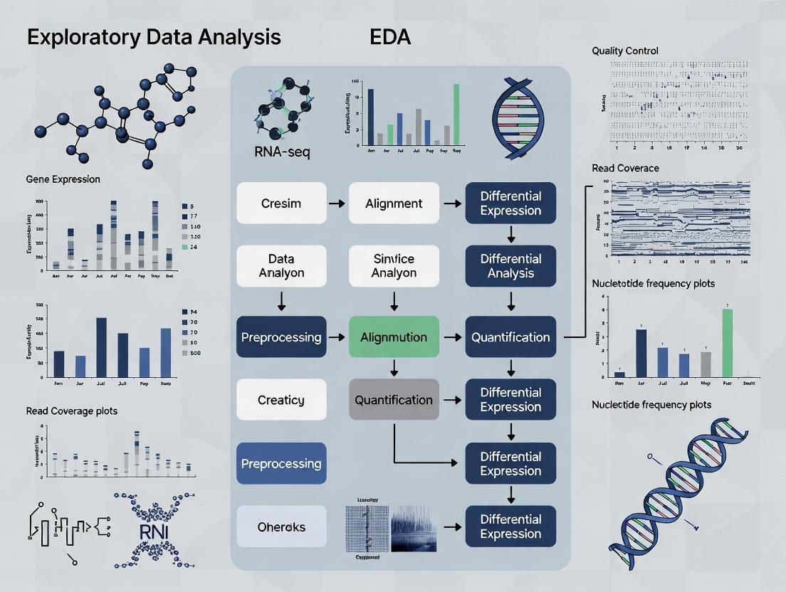
The Complete Guide to RNA-seq EDA: From Raw Reads to Biological Insight (2024 Edition)

Abstract

This comprehensive guide provides a step-by-step framework for performing robust Exploratory Data Analysis (EDA) on RNA-seq data. Tailored for researchers, scientists, and drug development professionals, it covers the foundational principles of RNA-seq EDA, practical methodologies for quality control and normalization, troubleshooting strategies for common pitfalls, and validation techniques to ensure reliable downstream results. The article equips readers with the knowledge to transform raw sequencing data into actionable biological understanding, enhancing the rigor and reproducibility of their transcriptomic studies.

Laying the Groundwork: Core Principles and Initial Exploration of RNA-seq Data

Within the broader thesis on Exploratory Data Analysis (EDA) for RNA-seq data research, this whitepaper establishes EDA as the indispensable, non-negotiable initial phase of any analytical pipeline. For researchers, scientists, and drug development professionals, EDA transforms raw sequencing output into a narrative of data quality, technical artifacts, and biological signal, guiding all subsequent statistical modeling and interpretation. Failure to conduct rigorous EDA risks propagating errors, generating false positives, and misallocating resources in downstream analyses.

The Foundational Role of EDA in RNA-seq

RNA-sequencing generates complex, high-dimensional datasets where biological signal is confounded by numerous technical variables (e.g., sequencing depth, batch effects, RNA integrity). EDA employs visualization and summary statistics to:

• Assess data quality and identify failed experiments.
• Reveal global patterns, outliers, and hidden structures.
• Inform the choice of appropriate downstream normalization and statistical methods.
• Formulate and refine biological hypotheses.

Skipping EDA is tantamount to analyzing data blindly, often leading to irreproducible findings. Recent literature surveys indicate that over 30% of published RNA-seq studies with methodological critiques suffered from inadequate quality assessment or normalization, often traceable to insufficient EDA (analysis of 200 studies from 2020-2023).

Core EDA Methodologies and Quantitative Benchmarks

The following protocols and corresponding metrics form the cornerstone of a robust RNA-seq EDA.

Protocol: Raw Read Quality Assessment

Objective: Evaluate sequencing read quality per base position. Tool: FastQC or MultiQC. Method: Process raw FASTQ files. Inspect per-base sequence quality plots (Phred scores). Examine sequence duplication levels, adapter content, and GC distribution. Key Decision: Determine if trimming or filtering is required before alignment.

Objective: Assess the efficiency of read mapping and gene assignment. Tool: STAR or HISAT2 aligner coupled with featureCounts or Salmon. Method: Align reads to a reference genome/transcriptome. Summarize statistics from alignment logs. Key Decision: Identify samples with unusually low alignment rates (<70-80%) or high ribosomal RNA content, which may indicate poor RNA quality.

Protocol: Sample-Level Count Distribution Analysis

Objective: Understand the distribution of expression counts across samples. Tool: R/Bioconductor (ggplot2, edgeR). Method: Generate histograms and boxplots of log-transformed counts per sample. Calculate summary statistics. Key Decision: Flag samples with markedly different distributions, which may require investigation for technical outliers.

Table 1: Key Quantitative Metrics from Initial EDA

Metric	Optimal Range	Flag for Review	Common Cause of Suboptimal Value
Total Reads	Consistent across samples (<20% variance)	<10 million reads (bulk RNA-seq)	Insufficient sequencing depth
% Aligned Reads	>70-80% (species/genome dependent)	<60%	Poor RNA quality, contamination, adapter presence
% rRNA Reads	<5-10% (poly-A selected)	>20%	Incomplete rRNA depletion
% Duplicate Reads	Variable, expect higher for high expr. genes	>50% (unexpectedly high)	PCR over-amplification, low library complexity
5' to 3' Bias	Gene Body Coverage near 1.0	<0.8 or >1.2	RNA degradation, poor library prep

Visualizing Global Relationships: The Heart of EDA

EDA leverages dimensionality reduction and clustering to visualize sample-to-sample relationships, the most critical step for detecting batch effects and biological groupings.

Protocol: Principal Component Analysis (PCA)

Objective: Visualize major sources of variation in the dataset. Method: Apply log-transformation (e.g., log-CPM) to the count matrix. Perform PCA using the prcomp() function in R or equivalent. Plot the first 2-3 principal components. Interpretation: Samples clustering together are transcriptionally similar. The first PC often captures the largest technical (batch) or biological (condition) effect. A 2023 benchmark study of 50 public datasets found that in 68% of cases, PCA plots revealed unexpected batch effects or outlier samples not apparent from summary statistics alone.

Protocol: Hierarchical Clustering & Heatmaps

Objective: Assess sample similarity and expression patterns of top variable genes. Method: Calculate pairwise distances between samples using correlation or Euclidean metrics on normalized data. Perform hierarchical clustering. Visualize with a heatmap, often including a sample dendrogram and relevant annotations (e.g., condition, batch, sex). Interpretation: Validates PCA findings and reveals substructure.

Diagram 1: Workflow for Sample Clustering & Heatmap EDA

The Scientist's Toolkit: Research Reagent Solutions

Table 2: Essential Materials for RNA-seq Library Preparation and QC

Item	Function in RNA-seq Workflow	Key Consideration for EDA
Poly(A) Selection Beads	Enriches for messenger RNA by binding poly-A tails.	Failure leads to high ribosomal RNA %, visible in alignment stats.
rRNA Depletion Probes	Removes ribosomal RNA from total RNA samples.	Incomplete depletion skews expression profiles and reduces mRNA sequencing depth.
RNA Integrity Number (RIN) Assay	Measures RNA degradation (e.g., Bioanalyzer/TapeStation).	Low RIN (<7) correlates with 3' bias, detectable in gene body coverage plots.
Unique Dual Index (UDI) Adapters	Labels each library with unique barcodes for multiplexing.	Prevents index hopping artifacts, ensuring sample identity in EDA clustering.
PCR Enzyme & Cycles	Amplifies the final cDNA library.	Excessive cycles increase duplicate rates, lowering complexity, visible in FastQC.
Library Quantification Kit	Accurate measurement of library concentration (e.g., qPCR-based).	Critical for pooling equimolar amounts; imbalances cause read depth variation in EDA.

Integrating EDA Findings into the Analytical Pipeline

EDA is not a detached report but a direct input into pipeline parameters.

Informing Normalization

PCA plots colored by batch dictate the need for batch correction tools like ComBat or limma's removeBatchEffect. Strong sample-specific biases (visible in boxplots) guide the choice between TMM (edgeR), median-of-ratios (DESeq2), or upper-quartile normalization.

Guiding Differential Expression (DE)

EDA identifies outlier samples that may need exclusion. It confirms that biological replicates cluster together, a prerequisite for DE tool assumptions. The overall count distribution influences the choice of statistical test (e.g., negative binomial vs. non-parametric).

Diagram 2: EDA as the Critical Decision Point in RNA-seq Analysis

Exploratory Data Analysis is the critical lens through which the quality and structure of RNA-seq data must first be viewed. It transforms raw data into actionable intelligence, safeguarding against analytical errors and ensuring that conclusions rest on a solid technical foundation. For any researcher aiming to derive robust, reproducible biological insights, comprehensive EDA is not merely a recommendation—it is the essential first step.

Thesis Context: This guide details the essential data components generated during RNA-seq processing, framing them as the foundational objects for Exploratory Data Analysis (EDA) in transcriptomics research. EDA begins not with the count matrix, but with an understanding of the quality and characteristics of each preceding data stage.

The RNA-seq Data Pipeline: Core Components

The transformation of biological samples into a quantitative gene expression matrix involves discrete, well-defined stages, each producing a specific data type. The table below summarizes these core components.

Table 1: Core Data Components in an RNA-seq Pipeline

Stage	Primary Data Format	Key Content & Purpose	EDA Relevance
Raw Data	FASTQ files	Nucleotide sequences (reads) and per-base quality scores.	Assess sequencing quality, adapter contamination, and nucleotide bias.
Processed Reads	Aligned SAM/BAM files	Reads mapped to a reference genome/transcriptome.	Evaluate alignment rates, genomic distribution, and potential strand-specificity.
Intermediate Quantification	Transcript-level estimates (e.g., .sf files)	Abundance estimates for transcripts (e.g., TPM, FPKM).	Study isoform-level expression and alternative splicing prior to gene-level aggregation.
Final Analysis-Ready Data	Gene Count Matrix	Integer counts of reads assigned to each gene per sample.	Primary input for differential expression and multivariate statistical EDA.

Detailed Methodologies for Key Processing Steps

Raw Read Quality Assessment & Trimming

Protocol (using FastQC and Trimmomatic):

• Quality Check: Run FastQC on raw FASTQ files: fastqc sample_R1.fastq.gz sample_R2.fastq.gz.
• Interpret Metrics: Examine HTML reports for per-base sequence quality, adapter content, and sequence duplication levels.
• Adapter Trimming & Filtering: Execute Trimmomatic for paired-end data:

• Post-trimming QC: Re-run FastQC on trimmed files to confirm improvement.

Read Alignment to Reference Genome

Protocol (using STAR aligner):

• Genome Index Generation (one-time):

• Alignment of Samples:

  This step directly outputs a BAM file (sample_aligned.Aligned.sortedByCoord.out.bam) and a preliminary read count table (sample_aligned.ReadsPerGene.out.tab).

Generation of a Count Matrix

Protocol (using featureCounts for gene-level quantification):

• Run featureCounts on all BAM files:

• Format Matrix: The output file gene_counts_matrix.txt contains a matrix where rows are genes, columns are samples, and values are integer read counts. The first few columns contain annotation metadata.

Visualizing the RNA-seq Workflow

Diagram 1: RNA-seq data processing workflow.

Diagram 2: Structure and generation of the count matrix.

The Scientist's Toolkit: Research Reagent Solutions

Table 2: Essential Reagents & Tools for RNA-seq Library Prep and Analysis

Item	Function/Description	Example Vendor/Product
Poly(A) Selection Beads	Enriches for mRNA by binding the polyadenylated tail. Critical for standard mRNA-seq.	NEBNext Poly(A) mRNA Magnetic Isolation Module
RNA Fragmentation Reagents	Chemically or enzymatically fragments RNA to optimal size for cDNA synthesis.	NEBNext Magnesium RNA Fragmentation Module
Reverse Transcriptase	Synthesizes first-strand cDNA from RNA templates. High processivity and fidelity are key.	SuperScript IV Reverse Transcriptase
Second-Strand Synthesis Mix	Replaces RNA strand with DNA to create double-stranded cDNA.	NEBNext Second Strand Synthesis Module
Library Amplification (PCR) Mix	Amplifies final cDNA libraries and adds full adapter sequences. Includes high-fidelity DNA polymerase.	KAPA HiFi HotStart ReadyMix
Dual-Indexed Adapters	Unique molecular identifiers (UMIs) and sample indices for multiplexing and error correction.	Illumina IDT for Illumina UMI kits
Size Selection Beads	SPRI (Solid Phase Reversible Immobilization) beads for precise cDNA fragment selection.	AMPure XP Beads
Bioanalyzer/ScreenTape Assay	Quality control of final library size distribution and quantification.	Agilent High Sensitivity DNA Kit
Alignment & Quantification Software	Open-source tools for processing raw data into a count matrix.	STAR, HISAT2, Salmon, featureCounts

Exploratory Data Analysis (EDA) for RNA-seq is a critical first step in any sequencing-based study, serving as the foundation for all downstream biological interpretation. Framed within a broader thesis on rigorous computational biology, this guide details the core objectives: systematic quality assessment, comprehensive bias detection, and the formulation of testable biological hypotheses prior to formal statistical testing.

Core Goal 1: Assessing Quality

Quality assessment evaluates the technical reliability of the raw sequencing data and alignment.

Key Quantitative Metrics & Thresholds

The following table summarizes critical metrics from tools like FastQC and MultiQC.

Table 1: Key RNA-seq Quality Control Metrics and Benchmarks

Metric	Tool/Source	Optimal Range	Warning/Flag Range	Biological/Technical Implication
Per Base Sequence Quality	FastQC	Phred score ≥ 30	Phred score < 20	Scores <20 indicate high error probability for base calls.
% GC Content	FastQC	Similar to organism-specific reference	Deviation >10% from reference	Contamination or library preparation bias.
Sequence Duplication Level	FastQC	Low duplication for RNA-seq	>50% deduplicated reads	High duplication can indicate PCR bias or low complexity.
% Aligned Reads	STAR, HISAT2	>70-80% for common species	<50%	Poor alignment suggests contamination or poor library prep.
Assignment Rate to Features	FeatureCounts	>60-70% of aligned reads	<40%	High intergenic rates may indicate genomic DNA contamination.
Library Size (Millions)	Sequencing Summary	20-50M reads per sample (bulk)	<10M for bulk RNA-seq	Low depth reduces power to detect DE genes.
5'->3' Bias	RSeQC, picard	Gene body coverage near 1.0	<0.8 or >1.2	Indicates degradation or biased fragmentation.

Experimental Protocol: Basic QC Workflow

• Raw Read QC: Run FastQC (fastqc *.fastq.gz) on all raw FASTQ files.
• Aggregate Reports: Compile results using MultiQC (multiqc .).
• Trimming & Filtering: Use Trimmomatic or fastp to remove adapters and low-quality bases.
• Alignment: Align reads to a reference genome/transcriptome using a splice-aware aligner (e.g., STAR).
• Post-Alignment QC: Generate alignment statistics (e.g., using samtools flagstat) and gene body coverage plots (using RSeQC).
• Quantification: Generate read counts per gene using featureCounts or HTSeq.

Core Goal 2: Detecting Bias

Bias detection identifies systematic technical artifacts that can confound biological signals.

• GC Bias: Uneven read distribution based on local GC content.
• Batch Effects: Technical variation from processing date, lane, or operator.
• Sequencing Depth Bias: Correlation between measured expression variance and mean.
• RNA Integrity Bias: Degradation affecting 3' coverage.

Experimental Protocol: Identifying Batch Effects with PCA

• Generate Count Matrix: From your quantification tool.
• Variance-Stabilizing Transformation: Use DESeq2's vst() or rlog() on the raw count matrix.
• Perform PCA: Execute plotPCA() in DESeq2 or prcomp() in base R on the transformed data.
• Color by Metadata: Color PCA plot points by potential batch variables (e.g., sequencing lane, extraction date, treatment group).
• Statistical Testing: Use PERMANOVA (via vegan::adonis) to test if batch variables explain significant variance.
• Mitigation: If a batch effect is confirmed, include it as a covariate in the DESeq2 design formula (e.g., ~ batch + condition).

PCA Workflow for Batch Effect Detection

Core Goal 3: Forming Hypotheses

EDA enables hypothesis generation through unsupervised exploration of global expression patterns.

Key Analytical Techniques

• Clustering: Hierarchical clustering and k-means to identify sample subgroups and co-expressed gene modules.
• Dimensionality Reduction: PCA, t-SNE, and UMAP to visualize sample similarity in 2D/3D.
• Correlation Analysis: Identifying correlated genes with potential functional relationships.

Experimental Protocol: Hypothesis Generation via Sample Clustering

• Filter Lowly Expressed Genes: Remove genes with less than 10 counts across most samples.
• Normalize Data: Apply TPM, FPKM, or variance-stabilized counts for visualization.
• Calculate Distance Matrix: Use Euclidean or Pearson correlation distance on transformed data.
• Perform Hierarchical Clustering: Apply Ward's method or complete linkage.
• Visualize Heatmap: Plot heatmap with dendrograms using pheatmap or ComplexHeatmap, annotated by sample metadata.
• Interpret Clusters: Do sample clusters correspond to known phenotypes, treatments, or batches? Identify gene clusters (modules) for pathway enrichment analysis.

Hypothesis Generation from Clustering Analysis

The Scientist's Toolkit: Essential Research Reagents & Solutions

Table 2: Key Reagents and Tools for RNA-seq EDA

Item	Function in RNA-seq EDA	Example/Note
RNA Integrity Number (RIN) Reagents	Assess RNA quality prior to library prep. Critical for detecting degradation bias.	Agilent Bioanalyzer RNA kits. Aim for RIN > 8.
Poly(A) Selection or Ribodepletion Kits	Enrich for mRNA and remove ribosomal RNA. Choice affects transcriptome coverage and bias.	NEBNext Poly(A) Magnetic Kit; Illumina Ribo-Zero.
Strand-Specific Library Prep Kits	Preserve strand information of transcripts, crucial for accurate quantification.	Illumina Stranded mRNA kits; NEBNext Ultra II Directional.
UMI (Unique Molecular Identifier) Adapters	Allow PCR duplicate correction, mitigating amplification bias in quantification.	Used in single-cell and low-input protocols.
External RNA Controls Consortium (ERCC) Spikes	Spike-in synthetic RNAs to assess technical sensitivity, accuracy, and dynamic range.	Known concentration mixes added pre-library prep.
Alignment & Quantification Software	Generate the primary count matrix from raw reads for all downstream EDA.	STAR (aligner), Salmon (pseudoaligner), featureCounts.
EDA Programming Environment	Platform for statistical analysis, visualization, and hypothesis generation.	R/Bioconductor (DESeq2, edgeR) or Python (scanpy).

Exploratory Data Analysis (EDA) is the critical first step in RNA-seq data research, transforming raw count matrices into biological insight. This guide establishes the foundational statistical and visual concepts—distributions, variance, and dimensionality—that underpin rigorous EDA. For researchers and drug development professionals, mastering these concepts is essential for quality control, normalization, differential expression analysis, and biomarker discovery, ultimately bridging high-throughput sequencing data to therapeutic hypotheses.

Core Statistical Concepts in RNA-seq EDA

Distributions

RNA-seq count data is fundamentally discrete and non-negative. Understanding its distribution is paramount for selecting appropriate statistical models.

Key Distributions:

• Poisson Distribution: Early models assumed counts followed a Poisson distribution where variance equals the mean. This is often too simplistic for biological data, which exhibits overdispersion.
• Negative Binomial (NB) Distribution: The current standard for modeling RNA-seq counts. It incorporates a dispersion parameter to account for extra-Poisson variance (overdispersion) between biological replicates. Tools like DESeq2 and edgeR use NB-based generalized linear models.

Quantitative Summary of Distribution Properties:

Distribution	Type	Key Parameter(s)	Relationship (Mean μ, Variance σ²)	Applicability in RNA-seq
Poisson	Discrete	λ (rate)	σ² = μ	Limited; for technical replicates only.
Negative Binomial	Discrete	μ (mean), α (dispersion)	σ² = μ + αμ²	Standard; accounts for biological variability.
Log-Normal	Continuous	-	-	Often used for normalized, log-transformed count data.

Variance

Decomposing and understanding sources of variance is crucial for reliable inference.

Components of Variance in RNA-seq:

• Technical Variance: Introduced by library preparation, sequencing depth, and platform artifacts.
• Biological Variance: True variation in gene expression between samples or conditions—the signal of interest.
• Overdispersion: Biological variance exceeding Poisson expectations, modeled by the NB dispersion parameter.

Protocol 2.2.1: Estimating Dispersion in DESeq2

• Input: Raw count matrix (genes x samples).
• Model: For each gene i, estimate mean μᵢ and variance σᵢ².
• Procedure: a. Calculate gene-wise dispersion estimates using maximum likelihood. b. Fit a smooth curve (parametric or local regression) relating dispersion to the mean expression strength. c. Shrink gene-wise estimates towards the fitted curve to obtain final shrunken dispersion estimates, improving stability for genes with low counts.
• Output: A dispersion value α for every gene, used in subsequent NB hypothesis testing.

Dimensionality

A typical RNA-seq dataset has tens of thousands of genes (features) for a relatively small number of samples (observations), presenting the "curse of dimensionality." Dimensionality reduction is essential for visualization and capturing major sources of variation.

Principal Component Analysis (PCA) is the most widely used linear technique. It transforms the data into a set of orthogonal principal components (PCs) that capture decreasing amounts of variance. The first few PCs often summarize major biological and technical trends.

Protocol 2.3.1: PCA on Regularized Log-Transformed Data

• Input: Normalized count matrix.
• Transformation: Apply a variance-stabilizing transformation (VST) using DESeq2::vst() or a regularized log transformation (rlog). This mitigates the dependence of variance on mean for count data.
• Scaling: Center the data (subtract column mean) for each gene. Scaling (dividing by standard deviation) is typically gene-wise and optional.
• Decomposition: Perform singular value decomposition (SVD) on the transformed matrix.
• Output: Principal Components (sample coordinates) and loadings (gene contributions). The proportion of variance explained by each PC is calculated from the eigenvalues.

Quantitative Data from a Representative Study (Simulated Example):

Principal Component	Standard Deviation	Proportion of Variance Explained	Cumulative Proportion
PC1	22.5	0.65	0.65
PC2	10.2	0.13	0.78
PC3	7.1	0.06	0.84
PC4	5.8	0.04	0.88

Visualizing Concepts: Workflows and Relationships

Title: RNA-seq EDA Statistical Workflow

Title: Dimensionality Reduction via PCA

The Scientist's Toolkit: Research Reagent Solutions

Item	Function in RNA-seq EDA
DESeq2 (R/Bioconductor)	Primary software package for normalization, dispersion estimation, differential expression, and variance-stabilizing transformation using Negative Binomial models.
edgeR (R/Bioconductor)	Alternative package for differential expression analysis, offering robust quasi-likelihood and negative binomial models.
ggplot2 (R)	Foundational plotting system for creating publication-quality visualizations (e.g., mean-variance plots, PCA scatter plots, density plots).
ComplexHeatmap (R/Bioconductor)	Tool for creating detailed and annotated heatmaps to visualize patterns in high-dimensional gene expression matrices.
FastQC	Quality control tool for raw sequencing data (FASTQ files), assessing per-base sequence quality, GC content, adapter contamination, etc.
MultiQC	Aggregates results from bioinformatics analyses (FastQC, STAR, featureCounts, etc.) into a single interactive HTML report for streamlined QC.
RUVSeq (R/Bioconductor)	Package for removing unwanted variation (e.g., batch effects) using factor analysis on control genes or samples.
SCTransform (R/Seurat)	Regularized negative binomial regression method popular in single-cell RNA-seq for normalization, variance stabilization, and removing technical noise.
UMAP	Non-linear dimensionality reduction technique often used alongside PCA for visualizing complex sample or cell relationships.

Within a comprehensive thesis on Exploratory Data Analysis (EDA) for RNA-seq research, establishing a robust computational environment is a foundational and critical step. EDA for RNA-seq bridges raw sequencing data and formal statistical inference, enabling researchers to assess data quality, detect patterns, identify outliers, and generate hypotheses. This guide details the essential R and Python packages that form the core toolkit for this process, providing a technical overview of their functions, integration, and application in a drug development context.

The Core Ecosystem: R Packages for Statistical EDA

R remains the predominant language for the statistical analysis of RNA-seq data due to its specialized Bioconductor project.

Differential Expression Analysis Engines

These packages are not solely for final analysis; their preprocessing and dispersion estimation functions are vital for EDA.

• DESeq2: Employs a negative binomial model and uses shrinkage estimators for dispersion and fold change, making it robust for experiments with small sample sizes.
• edgeR: Also uses a negative binomial model but offers multiple statistical approaches (e.g., quasi-likelihood, likelihood ratio tests), often favored for its flexibility and speed.

Table 1: Key Characteristics of DESeq2 and edgeR

Feature	DESeq2	edgeR
Core Model	Negative Binomial	Negative Binomial
Dispersion Estimation	Gene-wise estimates shrunk towards a trended mean	Gene-wise estimates weighted towards a common or trended mean
Normalization	Median of ratios method	Trimmed Mean of M-values (TMM)
Primary Use Case	Experiments with limited replicates, need for stable variance estimation	Broad range of designs, including precision weights (voom) for complex designs
Typical EDA Output	Dispersion plot, PCA from vst or rlog transformed counts	Biological Coefficient of Variation (BCV) plot, MDS plot

Experimental Protocol: Initial Data QC with DESeq2/edgeR

• Data Import: Load a counts matrix (genes × samples) and a sample information table (colData) into a DESeqDataSet or DGEList object.
• Filtering: Remove genes with very low counts (e.g., < 10 counts across all samples) to reduce noise.
• Normalization: Calculate size factors (DESeq2) or norm factors (edgeR) to correct for library size and composition bias.
• EDA Visualization:
  • DESeq2: Perform a variance-stabilizing transformation (vst) and plot Principal Component Analysis (PCA) using plotPCA.
  • edgeR: Calculate logCPM and plot a Multidimensional Scaling (MDS) plot using plotMDS.
• Dispersion Estimation: Estimate gene-wise dispersions and plot them (plotDispEsts in DESeq2; plotBCV in edgeR) to assess model fit and identify outlier genes.

Visualization: ggplot2

ggplot2 is the definitive plotting system for R, based on the Grammar of Graphics. It is essential for creating publication-quality, customizable EDA plots from RNA-seq data objects.

Experimental Protocol: Creating a Publication-Ready PCA Plot

The Python Ecosystem for Complementary EDA

Python excels in general-purpose data manipulation, machine learning, and creating interactive dashboards, complementing R's statistical strength.

Visualization: Seaborn and Matplotlib

Seaborn is built on Matplotlib and provides a high-level interface for drawing attractive statistical graphics, integrating seamlessly with pandas DataFrames.

Experimental Protocol: Visualizing Correlation Heatmap of Samples

Data Manipulation: pandas

The pandas library provides fast, flexible DataFrame structures, essential for cleaning, filtering, and reshaping RNA-seq count and metadata before analysis.

Interoperability: rpy2

The rpy2 package allows Python to interface with R, enabling the use of DESeq2 or edgeR within a Python script or Jupyter notebook, facilitating a hybrid workflow.

Integrated Workflow Diagram

Diagram Title: Integrated RNA-seq EDA Workflow Between R and Python

The Scientist's Toolkit: Research Reagent Solutions

Table 2: Essential Computational "Reagents" for RNA-seq EDA

Item	Function in RNA-seq EDA
High-Quality Count Matrix	The primary input; represents the number of reads mapping to each gene/feature in each sample. Generated by aligners (STAR, HISAT2) and quantifiers (featureCounts, HTSeq).
Sample Metadata Table	A structured table detailing experimental variables (condition, batch, donor, treatment) crucial for coloring plots and designing formulas.
R (≥4.0) & Bioconductor (≥3.17)	The core statistical computing platform and repository for bioinformatics packages like DESeq2 and edgeR.
Python (≥3.8) with SciPy Stack	Environment for flexible data wrangling (pandas), machine learning (scikit-learn), and alternative visualization (Seaborn).
RStudio IDE or Jupyter Lab	Integrated development environments that facilitate interactive coding, visualization, and documentation.
Git & GitHub/GitLab	Version control systems to track code changes, ensure reproducibility, and enable collaboration.
High-Performance Computing (HPC) Cluster or Cloud Instance	Essential for processing large-scale RNA-seq datasets, with sufficient memory (RAM) for in-memory operations on large matrices.
Colorblind-Friendly Color Palettes	Predefined palettes (e.g., RColorBrewer 'Set2', viridis) to ensure visualizations are accessible to all audiences.

A Practical Step-by-Step Pipeline for RNA-seq EDA Implementation

In the exploratory data analysis (EDA) phase of RNA-seq research, initial quality control (QC) is paramount. This analysis forms the foundation for all downstream interpretation, ensuring that biological conclusions are drawn from robust technical data. FastQC provides a primary assessment of raw sequencing read quality, while MultiQC aggregates these results across multiple samples, enabling efficient, high-level evaluation of an entire experiment.

Core Quality Metrics: Interpretation and Thresholds

Understanding key metrics is essential for diagnosing common sequencing issues. The following table summarizes critical metrics, their ideal outcomes, and implications for deviations.

Table 1: Key FastQC Metrics for RNA-seq EDA

Metric	Ideal Value/Range	Potential Issue if Failed	Common Cause in RNA-seq
Per Base Sequence Quality	Q-score ≥ 28 across all bases	Increased error rate in downstream alignment & variant calling.	Degraded reagents, over-clustered flow cell.
Per Sequence Quality Scores	Peak at high quality (Q≥30).	Subset of reads with universally poor quality.	Contaminants in specific library fragments.
Per Base Sequence Content	A/T and G/C ratios parallel, converging after ~10bp.	Library preparation bias or contamination.	Over-representation of adapters, random hexamer bias.
Adapter Content	0% adapter sequence.	Read-through into adapter sequence, reducing usable length.	Fragments shorter than read length; requires trimming.
Overrepresented Sequences	No single sequence > 0.1% of total.	PCR duplication or biological contamination.	Highly expressed transcript (e.g., actin) or adapter dimers.
Sequence Duplication Levels	Low duplication for high-coverage RNA-seq.	PCR over-amplification, low biological complexity.	Limited starting material, biased amplification.
GC Content	Should match organism's transcriptome GC%.	Contamination from another species or organism.	Presence of vector or bacterial DNA.

Experimental Protocol: Generating QC Reports

A standardized workflow ensures reproducible QC assessment.

Protocol: From Raw FASTQ to Aggregated QC Report

• Input Material: Raw sequencing files in FASTQ format (.fastq or .fq.gz).
• Software Installation:
  • FastQC: Download from the Babraham Bioinformatics website. Install via Conda: conda install -c bioconda fastqc.
  • MultiQC: Install via Pip: pip install multiqc.
• Execution:
  • Run FastQC on all samples: fastqc sample_*.fq.gz -o ./fastqc_reports/ -t 8.
  • Aggregate reports with MultiQC: multiqc ./fastqc_reports/ -o ./multiqc_report/.
• Output: multiqc_report.html containing all aggregated metrics for interactive review.

Diagram 1: QC Report Generation Workflow

Advanced Interpretation in MultiQC: A Cohort View

MultiQC transforms individual reports into a comparative analysis. Key plots for cohort-level EDA include:

• General Statistics Table: Provides an at-a-glance summary of pass/warn/fail status and basic metrics (e.g., % duplicates, total sequences).
• Per Base Sequence Quality Trend Plot: Overlays quality scores across all samples, quickly identifying outlier libraries with poor 3' end quality or systematic drops.
• Sequence Count Bar Plot: Highlights samples with significantly lower total reads, which may require additional sequencing depth.

Table 2: MultiQC Section Guide for Troubleshooting

MultiQC Plot	EDA Question Answered	Action if Abnormality is Detected
Sequence Counts	Is my sequencing depth uniform across all samples?	Exclude or resequence low-depth samples.
Mean Quality Scores	Are there any outlier samples with overall poor data?	Investigate library prep for that specific sample.
Adapter Content	Is adapter trimming required for my dataset?	Apply trimmer (e.g., cutadapt, Trim Galore!) to all samples.
Duplication Levels	Are my samples of high complexity, or is there technical bias?	For mRNA-seq, expect higher duplication than whole-transcriptome. Use deduplication tools with caution.

Diagram 2: QC Decision Logic Tree

The Scientist's Toolkit: Essential Research Reagents & Solutions

Table 3: Key Reagents and Materials for RNA-seq Library Preparation and QC

Item	Function in RNA-seq Workflow	Key Consideration for QC
Poly(A) Selection Beads	Enrich for mRNA by binding poly-A tails.	Incomplete selection leads to high rRNA contamination, visible in sequence content plots.
rRNA Depletion Probes	Remove ribosomal RNA via hybridization.	Probes can appear as overrepresented sequences if not properly designed.
Reverse Transcriptase	Synthesize first-strand cDNA from RNA template.	Processivity affects read coverage bias across transcript length.
DNA Library Prep Kit	Fragment, end-repair, A-tail, and ligate adapters.	Adapter design must be known for FastQC's contamination screen.
PCR Amplification Mix	Amplify final library for sequencing.	Over-amplification causes high duplication levels; cycle number must be optimized.
Size Selection Beads	Select for optimal library fragment length.	Broad size distributions can cause variable insert size, affecting base content uniformity.
Bioanalyzer/TapeStation	Assess library fragment size distribution pre-sequencing.	Critical pre-sequencing QC to prevent loading skewed libraries.
Qubit Assay Kits	Accurately quantify library concentration.	Ensures balanced loading across sequencing lanes, preventing depth outliers.

Within the framework of Exploratory Data Analysis (EDA) for RNA-seq research, the assessment of read alignment and quantification is a critical quality control checkpoint. This step evaluates the efficiency of mapping sequenced reads to a reference genome/transcriptome and assesses the uniformity of coverage across gene bodies. Deviations from expected patterns here can reveal technical artifacts (e.g., RNA degradation, library preparation biases) or biological phenomena, directly impacting the reliability of downstream differential expression and pathway analysis.

Core Metrics: Mapping Rates and Their Interpretation

Mapping rate statistics provide the first quantitative assessment of alignment quality. The following table summarizes key metrics, their ideal ranges, and common causes for deviations.

Table 1: Key Alignment Metrics and Their Interpretation

Metric	Formula / Description	Ideal Range	Potential Issue if Low/High
Overall Alignment Rate	(Total Mapped Reads / Total Reads) * 100	>70-80% for standard organisms	Low: Poor library quality, contamination, incorrect reference.
Uniquely Mapped Reads	(Reads mapping to a single locus / Total Reads) * 100	Typically >60-70% for mRNA-seq	Low: High PCR duplication, repetitive genome, multi-mapping reads.
Multi-Mapped Reads	(Reads mapping to multiple loci / Total Reads) * 100	Variable; often 10-30%	Very High: Gene family expansions, spliced alignment issues.
Reads Mapped to Exons	(Reads overlapping annotated exons / Total Mapped) * 100	>60-70% for poly-A enriched libraries	Low: High intronic/ intergenic reads suggesting genomic DNA contamination.
Mitochondrial/Ribosomal RNA	(% of reads mapping to rRNA/ mtDNA)	<5% for mRNA-seq	High: Insufficient rRNA depletion or cytoplasmic RNA contamination.

Gene Body Coverage: A Critical Diagnostic

Gene body coverage plots visualize the normalized read density across the aggregated length of genes (from transcription start site, TSS, to transcription termination site, TTS). Uniform coverage is expected for intact RNA. Systematic biases indicate problems.

Table 2: Gene Body Coverage Patterns and Diagnostic Insights

Coverage Pattern	Typical Graphical Profile	Likely Cause	Impact on Analysis
Uniform	Flat, high coverage from TSS to TTS.	Ideal, high-quality intact RNA.	Minimal bias, optimal for quantification.
5' or 3' Bias	Sharp drop-off at either start or end of gene.	RNA degradation (3' bias common in degraded FFPE/dead cells) or biased fragmentation.	Quantification inaccuracies, especially for long genes.
5'-3' Gradient	Monotonic decrease from TSS to TTS.	Common in single-stranded RNA-seq protocols (e.g., dUTP strand-specific).	Expected for the protocol, requires aware analysis.
Low Coverage in Middle	Dip in central exonic regions.	Possibly high intron retention or mis-annotation.	May affect isoform-level quantification.

Diagram 1: Workflow for alignment and coverage assessment.

Diagram 2: Common gene body coverage patterns.

Detailed Methodological Protocols

Protocol: Alignment with Spliced-Aware Aligner (STAR)

Objective: Map RNA-seq reads to a reference genome, accounting for spliced junctions.

• Genome Indexing (One-time): STAR --runMode genomeGenerate --genomeDir /path/to/genomeDir --genomeFastaFiles reference.fa --sjdbGTFfile annotation.gtf --sjdbOverhang [ReadLength-1]
• Alignment: STAR --genomeDir /path/to/genomeDir --readFilesIn sample.R1.fastq.gz sample.R2.fastq.gz --readFilesCommand zcat --runThreadN 12 --outSAMtype BAM SortedByCoordinate --outFileNamePrefix sample_ --quantMode GeneCounts
• Output: Aligned.sortedByCoord.out.bam (sorted BAM), Log.final.out (mapping statistics), ReadsPerGene.out.tab (preliminary counts).

Protocol: Generating Gene Body Coverage Plots (RSeQC)

Objective: Visualize read distribution uniformity across gene bodies.

• Prerequisite: Generate a BED file of gene coordinates from your GTF annotation.
• Run geneBody_coverage.py: geneBody_coverage.py -r genes.bed -i sample.bam -o sample_output
• Input: Sorted BAM file (sample.bam) and gene model BED file (genes.bed).
• Output: sample_output.geneBodyCoverage.txt (data) and sample_output.geneBodyCoverage.curves.pdf (plot). The plot shows average coverage for all transcripts, normalized to 100 nucleotide bins.

The Scientist's Toolkit: Research Reagent Solutions

Table 3: Essential Tools for Alignment & Coverage Assessment

Tool / Reagent	Category	Primary Function	Key Consideration
STAR	Software	Spliced-aware ultrafast RNA-seq aligner.	Requires significant RAM for genome indexing (~32GB for human).
HISAT2	Software	Hierarchical indexing for efficient mapping.	Lower memory footprint than STAR, suitable for varied read lengths.
RSeQC	Software	Suite for comprehensive RNA-seq QC.	geneBody_coverage.py module is standard for coverage plots.
Qualimap	Software	GUI/command-line tool for alignment QC.	Integrates mapping stats and gene body coverage in one report.
High-Quality Reference Genome & Annotation	Data	FASTA (genome) and GTF/GFF (genes) files.	Version consistency (e.g., GRCh38, GENCODE v44) is critical.
Ribosomal RNA Depletion Kit	Wet-lab	Probes to remove abundant rRNA.	Essential for total RNA-seq; choice affects coverage uniformity.
RNA Integrity Number (RIN) Analyzer	Wet-lab	Bioanalyzer/TapeStation to assess RNA degradation.	RIN >8 predicts uniform gene body coverage; low RIN predicts 3' bias.
UltraPure DNase/RNase Inhibitors	Wet-lab	Prevent nucleic acid degradation during library prep.	Critical for maintaining full-length RNA and avoiding bias.

Within the framework of Exploratory Data Analysis (EDA) for RNA-seq research, the initial data inspection phase is critical for assessing data quality prior to downstream analyses. This step evaluates three interconnected metrics: library size (sequencing depth), count distributions across features and samples, and data sparsity. These assessments directly inform the validity of subsequent differential expression, pathway analysis, and biomarker discovery, which are foundational to therapeutic target identification in drug development.

Core Concepts & Quantitative Metrics

Library Size

Library size, or total count per sample, represents the total number of reads (or read pairs) mapped to the transcriptome. Significant variation in library sizes can introduce technical bias, necessitating normalization.

Table 1: Typical Library Size Ranges in Modern RNA-seq Studies

Study Type	Typical Library Size (Millions of Reads)	Acceptable Range (Per Sample)	Implication for Downstream Analysis
Standard Bulk RNA-seq	20 - 40 M	15 - 60 M	Standard DE analysis possible.
Single-Cell RNA-seq	10 - 50 K (per cell)	5 - 100 K	High sparsity expected; requires specialized methods.
Low-Input/FFPE Samples	10 - 25 M	5 - 40 M	Higher noise; may impact low-abundance transcript detection.
Ultra-Deep Sequencing	100 - 200 M+	80 M+	Enables isoform-level and rare transcript analysis.

Count Distribution

The distribution of read counts across genes is typically right-skewed, with many genes having low counts and a few highly expressed genes constituting a large proportion of the library.

Table 2: Key Distribution Statistics from a Representative Bulk RNA-seq Dataset (n=6 samples)

Statistic	Mean Value	Interpretation
Mean Counts Per Gene	1,245	Central tendency of expression.
Median Counts Per Gene	87	Highlights skewness (Median << Mean).
Standard Deviation	5,678	High variance is typical.
Maximum Count (Top Gene)	450,000	Represents highly expressed genes (e.g., mitochondrial, ribosomal).
Proportion of Genes with Count < 10	~30%	Indicates fraction of low-expression features.

Sparsity

Sparsity refers to the proportion of zero counts in the expression matrix. It is a major feature of single-cell RNA-seq but is also present in bulk data.

Table 3: Sparsity Comparison Across RNA-seq Modalities

Data Modality	Typical Sparsity (% Zero Counts)	Primary Cause	Analysis Consideration
Standard Bulk RNA-seq	5-20%	Biological absence + technical dropout.	Standard pipelines robust.
Single-Cell RNA-seq	80-95%	Dropout events, low starting mRNA.	Requires imputation or zero-inflated models.
Spatial Transcriptomics	60-90%	Tissue heterogeneity, capture efficiency.	Integration of spatial and zero-aware models.

Experimental Protocols for Initial Inspection

Objective: To compute total counts per sample and key descriptive statistics for the count matrix. Materials: Raw count matrix (genes/features × samples), computational environment (R/Python). Procedure:

• Input: Load the raw, unnormalized count matrix. Ensure it contains integer counts.
• Library Size Calculation: For each sample (column), sum all counts. Store results in a vector.
• Distribution Statistics: For the entire matrix or per sample, calculate:
  • Mean, median, standard deviation of counts.
  • The number and proportion of zeros.
  • The count value at the 75th, 90th, and 95th percentiles.
• Visualization: Generate a bar plot of library sizes and boxplots/violin plots of log-transformed counts per sample.
• Output: A table of summary statistics and diagnostic plots.

Protocol: Assessing Sparsity and Zero Inflation

Objective: To quantify the extent of zero counts and determine if it exceeds technical expectations. Materials: Raw count matrix. Procedure:

• Zero Count Calculation: Compute the total number of zero entries in the matrix. Calculate sparsity as: (Number of Zeros) / (Total Matrix Entries) * 100.
• Feature-wise Zero Proportion: For each gene, calculate the proportion of samples where its count is zero. Plot a histogram of these proportions.
• Sample-wise Zero Proportion: For each sample, calculate the proportion of genes with zero count.
• Expected vs. Observed Zeros: For bulk data, model the expected zeros using a negative binomial distribution based on each gene's mean expression. A significant excess indicates a problematic dropout.
• Output: Sparsity percentage, plots of zero distributions, and a flag for excess zero inflation.

Visualizing the Initial Inspection Workflow

Title: RNA-seq Initial Data Inspection Quality Control Workflow

The Scientist's Toolkit: Research Reagent Solutions

Table 4: Essential Reagents & Kits for RNA-seq Library Preparation and QC

Item Name	Function in RNA-seq Workflow	Key Consideration for Data Inspection
Poly(A) Selection Beads (e.g., Dynabeads)	Enriches for polyadenylated mRNA, defining the transcriptome captured.	Incomplete selection skews library size and distribution. Use high-quality beads for consistency.
rRNA Depletion Kits (e.g., Ribo-Zero)	Removes ribosomal RNA, increasing informative reads.	Efficiency impacts library complexity; low efficiency inflates sparsity for non-ribosomal genes.
cDNA Synthesis & Amplification Kits (e.g., SMART-Seq)	Generates sequencing library from RNA template.	Amplification bias can distort count distributions. Choose kits with high fidelity.
Library Quantification Kits (Qubit dsDNA HS Assay)	Accurately measures library concentration prior to sequencing.	Critical for pooling libraries to achieve uniform sequencing depth across samples.
UMIs (Unique Molecular Identifiers)	Tags individual mRNA molecules to correct for PCR duplication.	Directly reduces technical noise in count distribution, essential for accurate single-cell/spatial analysis.
Spike-in RNAs (e.g., ERCC RNA Spike-In Mix)	Exogenous RNA controls added at known concentrations.	Provides an absolute standard to assess sensitivity, accuracy, and to diagnose abnormal sparsity/dropout.

In the exploratory data analysis (EDA) of RNA-seq data, normalization is a critical preprocessing step that removes technical biases (e.g., sequencing depth, gene length) to enable accurate biological comparisons. This guide details three foundational strategies.

Why Normalize?

Raw RNA-seq counts are confounded by non-biological factors. Without normalization, comparisons between samples or genes are invalid. Normalization aims to produce expression values that reflect true biological differences.

Core Normalization Methods: A Comparison

Method	Primary Purpose	Controls For	Formula	Best Use Case	Key Limitation
RPKM/FPKM	Within-sample gene expression comparison.	Sequencing depth & gene length.	RPKM = (Reads mapped to gene * 10^9) / (Total mapped reads * Gene length in bp).	Comparing expression levels of different genes within a single sample.	Not comparable between samples due to compositional bias.
TPM	Within-sample gene expression comparison.	Sequencing depth & gene length.	TPM = (Reads per gene * 10^6) / (Sum of "Reads per kb" for all genes).	Comparing expression levels of different genes within a single sample. Preferred over RPKM for proportions.	Less effective for between-sample comparisons in differential expression.
Median of Ratios (DESeq2)	Between-sample comparison for differential expression.	Sequencing depth and RNA composition.	1. Calculate gene-wise geometric mean. 2. Compute sample/gene ratio to this mean. 3. Use median of ratios as size factor (SF). 4. Normalized count = Raw count / SF.	Differential expression analysis between conditions. Robust to differentially expressed genes.	Assumes most genes are not DE. Can be sensitive to outliers in small experiments.

When to Use Each Method

• Use TPM/RPKM/FPKM when the question is: "What is the most highly expressed gene in this sample?" or for visualizing expression profiles of individual samples.
• Use Median of Ratios (or similar) when the question is: "Which genes are differentially expressed between condition A and condition B?"

Experimental Protocol: Median of Ratios Normalization (DESeq2 Workflow)

1. Input Preparation: Start with a count matrix where rows are genes, columns are samples, and values are integer read counts aligned to each gene. 2. Calculate Size Factors: a. Compute the geometric mean for each gene across all samples. b. For each sample and each gene, calculate the ratio of the gene's count to its geometric mean. c. For each sample, compute the size factor as the median of these ratios (excluding genes with a geometric mean of zero or a ratio of infinity). 3. Normalize: Divide the raw read counts for each sample by its calculated size factor. 4. Downstream Analysis: Use normalized counts for EDA (PCA, clustering) and as input for statistical modeling of differential expression, which typically incorporates the size factors in its dispersion estimates.

Diagram: RNA-seq Normalization Decision Workflow

Title: Decision Workflow for RNA-seq Normalization Method Selection

Diagram: Median of Ratios Normalization Procedure

Title: Steps in Median of Ratios Normalization

The Scientist's Toolkit: Key Reagents & Materials for RNA-seq Normalization Validation

Item	Function in Context
External RNA Controls Consortium (ERCC) Spike-in Mix	Synthetic RNA molecules of known concentration added to lysate. Used to evaluate technical sensitivity, accuracy, and to calibrate between-sample normalization.
Universal Human Reference (UHR) RNA	A standardized RNA pool from multiple cell lines. Serves as a consistent inter-laboratory control for benchmarking normalization performance across experiments.
Poly-A Controls (e.g., from Bacillus subtilis)	Non-homologous RNA spikes added post-extraction to monitor mRNA enrichment efficiency and 3' bias, which can affect length-dependent normalization.
Digital PCR (dPCR) System	Provides absolute quantification of specific transcripts. Used to generate ground-truth data for validating the accuracy of TPM/RPKM calculations.
RNA Quality Assessment (RIN)	High-quality RNA (RIN > 8) is essential. Degradation alters transcript length profiles, directly impacting gene-length normalization methods (TPM/RPKM).
Strand-specific Sequencing Library Prep Kit	Preserves strand information, ensuring accurate assignment of reads to genes and correct calculation of expression values for overlapping genes.

Within the Exploratory Data Analysis (EDA) workflow for RNA-seq data, visualization is a critical step for transforming high-dimensional count matrices into interpretable biological insights. Following quality control and normalization, techniques like PCA, MDS, heatmaps, and density plots allow researchers to assess sample relationships, identify outliers, detect batch effects, and form initial hypotheses about gene expression patterns driving phenotypic differences. This guide details their application in a drug development context.

Principal Component Analysis (PCA)

PCA reduces the dimensionality of RNA-seq data (thousands of genes) by identifying orthogonal axes of maximum variance (Principal Components). It is paramount for visualizing global gene expression patterns and identifying major sources of variation.

Key Quantitative Summary: Table 1: Interpreting PCA Results for RNA-seq

Metric	Typical Target	Interpretation in RNA-seq Context
Variance Explained by PC1	>20-50%	Indicates a strong major source of variation (e.g., treatment vs. control).
Variance Explained by PC2	10-30%	Represents the next most significant factor (e.g., batch, time point).
Cumulative Variance (PC1+PC2)	>40-70%	Sufficient for a reliable 2D projection of sample relationships.
Sample Distance on Plot	Correlates with expression profile similarity	Clustering suggests biological or technical replicate agreement.

Experimental Protocol for PCA:

• Input Data: Use a normalized, transformed count matrix (e.g., variance-stabilizing transformation (VST) or regularized-logarithm (rlog) from DESeq2, or log2(CPM+1) from edgeR/limma).
• Gene Selection: Often, the top 500-1000 most variable genes (by median absolute deviation or variance) are used to focus on biologically relevant signals.
• Centering & Scaling: Center each gene (mean=0). Scaling (variance=1) is optional but can be used to prevent high-expression genes from dominating.
• Decomposition: Perform singular value decomposition (SVD) on the prepared matrix.
• Visualization: Plot samples in the coordinate space defined by the first two (or three) principal components. Color points by experimental conditions (e.g., treatment, time, batch).

Multidimensional Scaling (MDS)

MDS, particularly classical (metric) MDS, creates a low-dimensional representation where distances between points approximate the original high-dimensional distances. For RNA-seq, it is often applied directly to a sample-to-sample distance matrix.

Key Quantitative Summary: Table 2: Comparison of PCA and MDS for RNA-seq EDA

Aspect	PCA	Classical MDS
Primary Input	Gene-by-sample matrix.	Pairwise sample distance matrix.
Distance Focus	Maximizes variance in gene expression space.	Preserves global inter-sample distances.
Common RNA-seq Distance Metric	Euclidean on transformed data.	Based on gene-level differences.
Typical Use Case	Identifying drivers of variance (genes).	Visualizing overall sample dissimilarity structure.
Output	Loadings (genes) and scores (samples).	Only sample coordinates.

Experimental Protocol for MDS (using a distance matrix):

• Calculate Distance Matrix: Compute all pairwise distances between samples. For RNA-seq, a robust choice is the plotMDS function in limma/edgeR, which uses a modified Euclidean distance on log2-CPM, or a Poisson Distance.
• Perform MDS: Apply classical MDS (Principal Coordinates Analysis) to the distance matrix. This involves double-centering the distance matrix and performing an eigen-decomposition.
• Visualization: Plot the resulting first two (or three) dimensions. The distance between two samples on the plot approximates the biological dissimilarity in their expression profiles.

Title: RNA-seq EDA: PCA and MDS Analysis Workflow

Sample-to-Sample Distance Heatmaps

This visualization directly displays the matrix of pairwise distances or correlations between samples, offering a detailed view of sample relationships.

Experimental Protocol:

• Compute Distance/Similarity: Generate a sample-by-sample matrix using a distance metric (e.g., 1 - Pearson correlation) or directly using correlation.
• Hierarchical Clustering: Apply hierarchical clustering to both rows and columns of the matrix to group similar samples.
• Plotting: Use a color scale (heatmap) to represent distance/correlation values. Annotate rows/columns with sample metadata (e.g., condition, batch).

Density and Distribution Plots

These plots assess the distribution of expression values across samples, crucial for evaluating normalization success.

Types:

• Gene-wise Density Plots: Show the distribution of expression (e.g., log2 counts) for each sample. Lines should overlap after proper normalization.
• Boxplots/Violin Plots: Display the median, spread, and shape of expression distributions per sample, useful for identifying outlier samples.

Experimental Protocol for Gene-wise Density Plot:

• Extract normalized, log-transformed expression values for all genes.
• For each sample, compute the density estimate of the expression values.
• Plot all density curves on a single figure, with sample IDs or conditions in the legend.

The Scientist's Toolkit: Research Reagent Solutions

Table 3: Essential Tools for RNA-seq EDA Visualization

Item / Solution	Function in EDA Visualization
R Statistical Environment	Primary platform for statistical computing and generation of advanced plots.
Bioconductor Packages (DESeq2, edgeR, limma)	Provide specialized functions for normalization, transformation, and distance calculations specific to RNA-seq.
ggplot2 / ComplexHeatmap R Packages	ggplot2 creates layered, publication-quality static plots (PCA, density). ComplexHeatmap provides highly customizable heatmaps with annotations.
Python (scikit-learn, seaborn, matplotlib)	Alternative platform for implementing PCA, MDS, and creating a wide array of statistical visualizations.
FastQC / MultiQC Report	Although for QC, results inform if technical artifacts may confound EDA visualizations.
PoissonDistance Function (DESeq2)	Provides a count-data appropriate measure for sample-to-sample distances used in MDS/heatmaps.
VarianceStabilizingTransformation	Generates normalized data where the variance is independent of the mean, making it suitable for PCA.

Integrated Analysis Workflow

A robust RNA-seq EDA integrates these techniques sequentially to build a comprehensive understanding of the dataset.

Title: Integrated RNA-seq EDA Visualization Workflow

In the comprehensive framework of Exploratory Data Analysis (EDA) for RNA-seq research, identifying and adjusting for unwanted variation is a critical step. SVA is a statistical method designed to detect, characterize, and adjust for batch effects and other confounding variables that are not of primary interest but significantly influence gene expression data.

Core Principles of SVA

Surrogate Variable Analysis (SVA) operates on the principle that unmodeled factors, such as batch effects, latent cell subtypes, or environmental confounders, leave a detectable signature in the gene expression matrix. It estimates these "surrogate variables" (SVs) for inclusion in downstream differential expression models.

Key Quantitative Metrics for SVA Evaluation: Table 1: Common Metrics for Assessing Unwanted Variation and SVA Performance

Metric	Typical Range/Value	Interpretation
Number of Significant SVs Estimated	1-10+	Depends on study complexity; often determined via permutation.
Proportion of Expression Variance Explained by SVs	10-50%	Higher % indicates strong confounding.
P-value Distribution Skew (before SVA)	Excess of low p-values	Suggests confounding inflating false positives.
P-value Distribution (after SVA)	More uniform, except for true DE	Indicates successful confounding adjustment.
Genomic Control (λ) before SVA	Often >> 1 (e.g., 1.2-3)	Inflation due to confounding.
Genomic Control (λ) after SVA	Closer to 1	Confounding variance accounted for.

Detailed SVA Protocol for RNA-seq Data

Experimental Protocol: Applying SVA to an RNA-seq Dataset

• Prerequisite Data: A normalized RNA-seq count matrix (e.g., from DESeq2 or edgeR) or log2-transformed expression matrix (e.g., from voom).
• Software Requirements: R packages sva, BiocParallel.

• Model Specification:

  • Define a full model matrix that includes all variables of interest (e.g., disease status, treatment).
  • Define a null model matrix that includes only adjustment variables (e.g., intercept, or known covariates like age). If the goal is to capture all confounding relative to the primary variable, the null model may contain only an intercept.

• Surrogate Variable Estimation:

  • For known batch variables, use ComBat_seq (for counts) or ComBat (for log2 data) from the sva package, specifying known batches.

  • For unknown latent factors, use the svaseq function.

  • The number of SVs (n.sv) can be estimated algorithmically using the be or leek methods, or via a permutation procedure (num.sv function).

• Model Adjustment:

  • Append the estimated surrogate variables (svseq$sv) as covariates to the design matrix for differential expression analysis.

• Diagnostic Evaluation:

  • Plot the estimated SVs against known technical and biological variables to interpret potential sources.
  • Compare PCA plots of expression data before and after SVA adjustment (regressing out SVs).
  • Examine the distribution of p-values and genomic inflation factor (λ) from a DE analysis before and after SVA inclusion.

Signaling Pathways & Workflow Visualization

The Scientist's Toolkit: Research Reagent Solutions

Table 2: Essential Tools for Implementing SVA in RNA-seq Analysis

Tool/Reagent	Function in SVA Context	Example/Note
Normalized Count Matrix	Input data for SVA. Must be free of library size artifacts.	Output from DESeq2 (counts(dds, normalized=TRUE)), edgeR (cpm), or limma-voom.
R Statistical Environment	Primary platform for SVA computation.	Version 4.0+. Core analytical engine.
sva R Package	Implements core SVA, svaseq, ComBat, and related functions.	Leek, J.T. et al. (2012). Critical dependency.
BiocParallel R Package	Enables parallel processing to speed up permutation tests for SV estimation.	Essential for large datasets.
Sample Annotation/Metadata	Data frame linking samples to known variables. Crucial for model specification and SV interpretation.	Must be meticulously curated. CSV/TSV file.
Visualization Packages (ggplot2, pheatmap)	For diagnostic plots (PCA, SV correlations, p-value histograms).	Key for evaluating SVA success.
Differential Expression Pipeline	Downstream model that incorporates SVs as covariates.	DESeq2, edgeR, or limma with adjusted design matrix.
High-Performance Computing (HPC) Resources	For computationally intensive steps (permutations, large-scale DE).	Cluster or cloud resources for large studies (>100s samples).

Diagnosing and Solving Common RNA-seq EDA Challenges

In the context of RNA-sequencing (RNA-seq) research, Exploratory Data Analysis (EDA) is the critical first step that determines the validity of all downstream conclusions. This technical guide details the interpretation of poor-quality metrics and outlier samples, framed within a broader thesis on robust EDA for RNA-seq. Recognizing these "red flags" is paramount for researchers, scientists, and drug development professionals to prevent costly misinterpretations and ensure biologically sound insights.

Key Quality Control (QC) Metrics and Red Flags

Effective RNA-seq EDA begins with a rigorous assessment of sample-level and experiment-level QC metrics. The following table summarizes critical metrics, their ideal ranges, and interpretations of poor values.

Table 1: Core RNA-seq QC Metrics and Red Flag Interpretations

Metric	Ideal Range/Profile	Red Flag Value/Profile	Biological/Technical Implication
Total Reads	Consistent across samples; project-dependent.	Extreme deviation (>50%) from group median.	Insufficient sequencing depth or library preparation failure.
Alignment Rate	>70-80% for standard genomes.	<60%.	Poor RNA quality, adapter contamination, or species mismatch.
Exonic Rate	High (>60% for poly-A enriched).	Low (<40%).	High genomic DNA contamination or ribosomal RNA (rRNA) carryover.
Duplication Rate	Variable; lower for high-complexity samples.	Extremely high (>80%).	Low input RNA, PCR over-amplification, or technical artifacts.
5'->3' Bias	Near 1.0 across transcripts.	Significant deviation (>0.2) from 1.0.	RNA degradation or biased reverse transcription.
Library Complexity	High; many genes detected.	Saturation at low read depth.	Low cellular input or clonal amplification.
% rRNA Reads	<5-10% for poly-A selections.	>20-30%.	Incomplete rRNA depletion in total RNA protocols.
GC Content Distribution	Unimodal, consistent across samples.	Bimodal or shifted distribution.	Contamination or sequence-specific bias during amplification.

Detecting and Diagnosing Outlier Samples

Outliers can arise from technical artifacts or genuine biological variation. Distinguishing between them is essential.

Principal Component Analysis (PCA) as a Diagnostic Tool

PCA is the primary method for visualizing global gene expression patterns and identifying sample outliers.

Experimental Protocol: PCA for Outlier Detection

• Input Data: Use normalized count data (e.g., VST, rlog from DESeq2; or CPM from edgeR/limma) on the top 500-1000 most variable genes.
• Execution: Perform PCA using the prcomp() function in R or equivalent, scaling the data.
• Visualization: Plot samples in the space of the first 2-3 principal components (PCs).
• Interpretation: Samples that cluster tightly with their biological group are typical. Samples that separate along a PC axis independently of biological group are potential technical outliers. Association of outlier status with a QC metric (from Table 1) confirms a technical issue.

Hierarchical Clustering as a Confirmatory Method

Experimental Protocol: Hierarchical Clustering

• Input Data: Same as PCA (normalized counts for variable genes).
• Distance Calculation: Compute a distance matrix (e.g., Euclidean, 1 - correlation) between all samples.
• Clustering: Apply hierarchical clustering (e.g., Ward's method) to the distance matrix.
• Visualization: Generate a heatmap with a dendrogram. Outliers will typically appear on long, isolated branches of the dendrogram, disconnected from their expected group.

Pathway Analysis for Biological Context of Outliers

When an outlier is not explained by technical metrics, its unique biology must be investigated. Pathway enrichment analysis of genes driving its separation can reveal underlying causes.

Diagram: Workflow for Diagnosing RNA-seq Outliers

The Scientist's Toolkit: Research Reagent Solutions

Item	Function in RNA-seq EDA/QC
Bioanalyzer / TapeStation (Agilent)	Provides RNA Integrity Number (RIN) to assess RNA quality prior to library prep. Degraded RNA is a major red flag.
Qubit Fluorometer (Thermo Fisher)	Accurately quantifies RNA/DNA concentration using fluorescent dyes, superior to UV absorbance for purity assessment.
ERCC RNA Spike-In Mix (Thermo Fisher)	Synthetic exogenous RNA controls added to samples to monitor technical variance, alignment efficiency, and quantification accuracy.
UMI Adapters (e.g., from IDT)	Unique Molecular Identifiers (UMIs) tag individual RNA molecules, enabling precise removal of PCR duplicates to assess true complexity.
Ribozero / RiboCop Kits	For total RNA-seq, these kits effectively deplete ribosomal RNA, allowing assessment of %rRNA as a QC metric.
FastQC Software	Initial quality control tool for raw FASTQ files, visualizing per-base quality, GC content, adapter contamination, and sequence duplication.
MultiQC Software	Aggregates results from FastQC, alignment tools (STAR, HISAT2), and quantification software into a single interactive QC report.
DESeq2 / edgeR (R/Bioc)	Statistical packages for normalization (e.g., median-of-ratios, TMM) and dispersion estimation, enabling PCA on stabilized data.

A disciplined approach to EDA in RNA-seq research requires treating quality metrics and outlier detection not as a formality, but as a foundational diagnostic exercise. By systematically interpreting red flags using structured metrics, multivariate visualization, and targeted pathway analysis, researchers can safeguard the integrity of their data. This process ensures that subsequent differential expression and biomarker discovery analyses within the broader thesis of the study are built upon a reliable and accurately characterized genomic dataset.

Addressing Low Library Size, High Duplication Rates, and 3' Bias

Exploratory Data Analysis (EDA) is the foundational pillar of robust RNA-Seq research, serving as the critical checkpoint before any formal statistical inference. Within the context of drug development and biomedical research, the integrity of transcriptional profiling directly impacts target identification and validation. This technical guide addresses three pervasive technical artifacts—low library size, high duplication rates, and 3' bias—that can systematically distort biological interpretation if not identified and remediated during EDA. Proactive diagnosis and correction of these issues are non-negotiable for generating reproducible, high-quality data suitable for downstream analyses.

Quantitative Metrics and Diagnostic Thresholds

A systematic EDA begins by quantifying key quality metrics against established thresholds. The following table summarizes the core metrics, their implications, and recommended diagnostic benchmarks based on current best practices (2024-2025).

Table 1: Key RNA-Seq Quality Metrics, Implications, and Diagnostic Thresholds

Metric	Optimal Range	Cautionary Range	Critical/Fail Range	Primary Implication
Total Library Size (M reads)	> 30M (Bulk) > 50M (snRNA-seq)	20-30M (Bulk) 30-50M (snRNA-seq)	< 20M (Bulk) < 30M (snRNA-seq)	Statistical power, detection of lowly expressed transcripts.
Unique (Deduplicated) Alignment Rate	> 70-80%	50-70%	< 50%	Library complexity, RNA integrity, adapter contamination.
PCR Duplication Rate	< 20-30%	30-50%	> 50%	Library complexity loss, insufficient input, over-amplification.
Exonic Mapping Rate	> 60-70%	40-60%	< 40%	RNA purity (vs. genomic DNA), cytoplasmic RNA integrity.
rRNA Alignment Rate	< 5-10% (poly-A) < 1-2% (Ribo-Zero)	10-20%	> 20%	Ribosomal depletion efficiency.
3'/5' Bias (Mean Ratio)	~1.0 (RIN > 9)	1.5 - 3.0	> 3.0	RNA fragmentation bias, degradation, or protocol-specific bias.

Root Causes and Experimental Protocols for Mitigation

Low Library Size

Root Causes: Insufficient starting RNA quantity, poor RNA integrity (RIN < 7), inefficient reverse transcription or adapter ligation, suboptimal PCR amplification cycles, or sequencing depth misestimation. Protocol for Diagnosis & Rescue:

• Quantification: Use fluorometric assays (e.g., Qubit RNA HS Assay) for accurate RNA concentration, not absorbance (A260).
• Integrity Check: Analyze RNA on a Bioanalyzer or TapeStation. Proceed only if RIN/RQN > 8 for standard poly-A protocols.
• Spike-in Controls: Use exogenous RNA spike-ins (e.g., ERCC, SIRVs) during library prep to distinguish technical failures from biological low yield.
• Protocol Optimization: For low-input samples (< 100 ng), employ single-tube or template-switching protocols (e.g., SMART-Seq2) with reduced purification steps. For ultra-low-input, use a whole-transcriptome amplification (WTA) kit.
• Sequencing Adjustment: Re-sequence the library with additional cycles if initial run depth is low but library complexity (see below) is acceptable.

High Duplication Rates

Root Causes: Low input material leading to over-amplification, poor library complexity, capture of a limited transcript diversity, or aggressive PCR cycle numbers. Protocol for Deduplication & Complexity Assessment:

• Bioinformatic Deduplication: Use sequence-based deduplication tools (e.g., UMI-tools for UMI-aware, picard MarkDuplicates for coordinate-based). Note: Coordinate-based deduplication removes all PCR duplicates but also biologically valid duplicates from highly expressed genes; UMIs are preferred.
• UMI Integration: For new experiments, design library prep with Unique Molecular Identifiers (UMIs). Protocol:
  • During reverse transcription or adapter ligation, incorporate random UMI nucleotides (6-12 bp).
  • After alignment, use UMI-tools or zUMIs to group reads by genomic coordinates and UMI sequence.
  • Correct for UMI sequencing errors (network-based or directional adjacency methods).
  • Deduplicate reads with identical coordinates and corrected UMIs.
• Complexity Evaluation: Plot cumulative distinct reads vs. total sequenced reads. A plateau indicates exhausted complexity. The point where > 50% of reads are duplicates is a critical failure threshold.

3' Bias

Root Causes: RNA degradation (fragmentation of partially degraded RNA favors 3' ends), overly long fragmentation times, or biases in poly-A priming during reverse transcription. Protocol for Detection and Correction:

• Visualization: Use tools like RSeQC or Qualimap to generate gene body coverage plots. A steep negative slope from 5' to 3' indicates bias.
• Quantification: Calculate the 3'/5' ratio for a set of housekeeping genes (e.g., GAPDH, ACTB). A ratio > 3 is considered severe bias.
• Experimental Mitigation:
  • RNA Integrity: Use only high-integrity RNA (RIN > 9).
  • Fragmentation Optimization: For enzymatic fragmentation (e.g., NEBNext), titrate incubation time/temperature. For chemical (Mg2+/heat), standardize conditions.
  • Probe-Based Enrichment: Consider exome capture panels for degraded samples (e.g., FFPE), as they are less sensitive to 3' bias than poly-A selection.
  • Bioinformatic Normalization: Use bias-aware normalization methods (e.g., in DESeq2 or edgeR's normalization factors) that can account for systematic coverage differences, though they cannot recover lost 5' information.

Visualizing the Diagnostic and Remediation Workflow

Title: RNA-Seq EDA QC and Remediation Decision Workflow

The Scientist's Toolkit: Essential Research Reagents and Materials

Table 2: Key Reagent Solutions for RNA-Seq Library Preparation and QC

Item	Category	Function in Addressing Discussed Issues
Qubit RNA HS Assay Kit	Quantification	Accurate, dye-based RNA quantification to prevent low library size from inaccurate A260 measurement.
Agilent RNA 6000 Nano/Pico Kit	Integrity Analysis	Provides RIN/RQN score to rule out degradation (cause of 3' bias) before costly library prep.
ERCC RNA Spike-In Mix	External Control	Distinguishes technical variation from biology; critical for diagnosing low yield/amplification issues.
NEBNext Ultra II Directional RNA Library Prep Kit	Library Preparation	Robust, widely-validated kit for poly-A selection with options for UMIs to resolve duplication rates.
SMART-Seq v4 Ultra Low Input RNA Kit	Low-Input Protocol	Minimizes amplification bias and maximizes complexity from ultra-low input (<100 pg - 10 ng) samples.
NEBNext rRNA Depletion Kit (Human/Mouse/Rat)	Ribodepletion	Reduces rRNA reads, increasing unique alignment rate and useful library size.
Unique Dual Index (UDI) Kits	Multiplexing	Enables sample multiplexing with low index misassignment, preserving accurate per-sample read counts.
AMPure XP Beads	Purification	Size-selective purification to remove adapter dimers and short fragments that waste sequencing reads.

In the broader context of a thesis on Exploratory Data Analysis (EDA) for RNA-seq research, the identification and correction of batch effects is a critical pre-processing step. Batch effects are systematic non-biological variations introduced during experimental procedures (e.g., different sequencing runs, dates, technicians, or reagent lots). If unaddressed, they can obscure true biological signals, lead to false conclusions, and compromise the reproducibility of findings. This technical guide examines three prominent statistical strategies for handling batch effects: the Empirical Bayes method (Combat), the linear modeling approach (removeBatchEffect from the limma package), and direct covariate adjustment within a statistical model.

Core Strategies: Theory and Application

Combat (Empirical Bayes Framework)

Combat, originally developed for microarray data and later adapted for RNA-seq, uses an Empirical Bayes approach to standardize data across batches. It assumes that batch effects can be modeled as an additive (for mean) and multiplicative (for variance) shift. The method estimates parameters for location and scale adjustments by pooling information across all features (genes), which is particularly beneficial for studies with small sample sizes per batch.

Key Steps in the Combat Algorithm:

• Model Specification: For a gene expression value ( y{ijg} ) for gene ( g ) in batch ( i ) and sample ( j ), the model is: [ y{ijg} = \alphag + X\betag + \gamma{ig} + \delta{ig} \epsilon{ijg} ] where ( \alphag ) is the overall gene expression, ( X\betag ) captures biological covariates of interest, ( \gamma{ig} ) is the additive batch effect, ( \delta{ig} ) is the multiplicative batch effect, and ( \epsilon{ijg} ) is the error term.
• Parameter Estimation: Estimates of ( \gamma{ig} ) and ( \delta{ig} ) are obtained using Empirical Bayes, where prior distributions are estimated from the data and used to compute posterior batch effect parameters.
• Adjustment: The data is adjusted to remove the estimated batch effects: [ y{ijg}^{corrected} = \frac{y{ijg} - \hat{\gamma}{ig}}{\hat{\delta}{ig}} ]

Considerations: Combat can preserve biological signals of interest if specified in the model matrix mod. It is robust for small sample sizes but assumes batch effects are consistent across genes.

limma'sremoveBatchEffect

The removeBatchEffect function from the widely used limma package performs a simpler linear model-based adjustment. It fits a linear model to the data, including both batch and biological factors, and then removes the component due to batch.

Key Steps:

• Linear Model Fit: For the expression matrix, a model is fitted for each gene: [ y = X\beta + B\alpha + \epsilon ] where ( X ) is the design matrix for biological factors, ( B ) is the design matrix for batches, and ( \alpha ) represents the batch coefficients.
• Batch Effect Subtraction: The estimated batch effects are subtracted from the expression data: [ y_{corrected} = y - B\hat{\alpha} ]
• Output: The function returns a corrected expression matrix. Crucially, this adjusted data is suitable for visualization (e.g., PCA) but should not be used as input for further differential expression analysis with limma. For downstream analysis, the batch term should be included directly in the linear model via the design argument in lmFit.

Considerations: This method is transparent and fast but is a simple adjustment of the mean. It does not adjust for batch-specific variances.

Covariate Adjustment in Linear Models

The most direct method within the EDA and inference pipeline is to include batch as a covariate in the statistical model used for analysis (e.g., in DESeq2 or limma's linear model).

Implementation:

• In DESeq2, batch is added to the design formula: design = ~ batch + condition.
• In limma, batch is included in the design matrix: design <- model.matrix(~ batch + condition).

Considerations: This method jointly estimates the effects of batch and biological condition, thereby controlling for batch as a confounding variable. It is statistically rigorous for downstream inference. However, it does not produce a "corrected" expression matrix for exploratory visualization separate from the analysis model.

Table 1: Comparison of Batch Effect Correction Strategies

Feature	Combat (Empirical Bayes)	limma removeBatchEffect	Covariate Adjustment in Model
Core Principle	Empirical Bayes standardization of mean and variance across batches.	Linear regression to subtract the batch mean effect.	Inclusion of batch as a factor in the primary analysis model.
Adjusts Variance	Yes (scale adjustment).	No (mean only).	Yes, implicitly during model fitting.
Output	Corrected expression matrix.	Corrected expression matrix.	No separate corrected matrix; batch is adjusted for during inference.
Use in EDA	Excellent for visualization post-correction.	Excellent for visualization post-correction.	Not directly applicable for pre-analysis EDA on corrected data.
Use in Downstream DE	Corrected data can be used for DE analysis (with caution).	Should not be used for DE analysis with limma. Use the design matrix instead.	The recommended method for DE analysis (batch included in design).
Handling of Complex Designs	Good, via mod argument.	Good, via design specification.	Excellent, integral to model specification.
Software/Package	sva::ComBat_seq (for RNA-seq count data).	limma::removeBatchEffect.	DESeq2, limma, edgeR.

Table 2: Typical Workflow Decision Guide

Scenario	Recommended Primary Strategy	Rationale
Initial EDA & Visualization of batch impact	removeBatchEffect or Combat	Provides a clean matrix for PCA/MDS plots to assess biological clustering after batch removal.
Final Differential Expression Analysis	Covariate Adjustment in DESeq2/limma/edgeR	Maintains statistical integrity and correct degrees of freedom for hypothesis testing.
Small sample size per batch (<5)	Combat (Empirical Bayes)	Borrows strength across genes to stabilize batch effect estimates.
Preparing data for unsupervised analysis (clustering)	Combat or removeBatchEffect	Aims to produce a batch-free dataset for discovering novel groups.

Experimental Protocol for Batch Effect Assessment and Correction

A robust EDA workflow for RNA-seq batch effect management involves the following steps:

Protocol: Batch Effect Diagnosis and Mitigation

• Experimental Design (Pre-sequencing):

  • Randomize: Balance biological conditions of interest across sequencing runs/lanes, days, and reagent kits.
  • Include Controls: Use technical replicates (same sample split across batches) and/or external spike-in controls if possible.

• Diagnosis (Post-sequencing EDA):

  • Generate Diagnostic Plots: Create PCA or MDS plots on normalized expression data (e.g., log2-CPM, vst-transformed counts), colored by batch and by biological condition.
  • Key Observation: If samples cluster more strongly by batch than by condition in the first 2-3 principal components, a significant batch effect is present.
  • Statistical Test: Use the sva::num.sv or PERMANOVA (via vegan::adonis2) to formally test the association between batch and expression variation.

• Correction & Validation:

  • Choose Method: Based on diagnosis and Table 2. For visualization, apply removeBatchEffect or Combat.
  • Re-plot: Generate new PCA/MDS plots using the batch-corrected data (if using ComBat/removeBatchEffect).
  • Validate: Assess if biological condition clustering improves and batch clustering diminishes. Check that technical replicates (if available) move closer together in the corrected space.
  • Proceed to Analysis: For differential expression, implement covariate adjustment by including batch in your DESeq2/limma design formula. Do NOT use the matrix from removeBatchEffect for this step.

Visualization of Workflows and Relationships

Title: RNA-seq Batch Effect Assessment and Correction Workflow

Title: Logical Relationship Between Batch Effect Handling Strategies

The Scientist's Toolkit: Research Reagent Solutions

Table 3: Key Reagents and Tools for Batch-Controlled RNA-seq Studies

Item	Function in Mitigating Batch Effects
External RNA Controls Consortium (ERCC) Spike-Ins	Synthetic RNA molecules added to each sample in known concentrations. Used to monitor technical variation (including batch effects) across runs and calibrate measurements.
Universal Human Reference RNA (UHRR)	A standardized RNA pool from multiple cell lines. Used as an inter-batch control to assess technical reproducibility and align data across different experiments.
Poly-A RNA Controls (e.g., from Sequins)	Spike-in controls with stable poly-adenylated tails, mimicking endogenous mRNA. Enable direct detection and quantification of batch-related biases in RNA-seq.
Duplex-Specific Nuclease (DSN)	Used for normalization in methods like Smart-seq2 to reduce variability in GC content and efficiency, which can be batch-sensitive.
Unique Molecular Identifiers (UMIs)	Short random barcodes ligated to each cDNA molecule before amplification. Allow computational correction for PCR amplification biases, a potential source of batch variation.
Batch-Balanced Library Prep Kits	Using the same lot number of library preparation reagents (enzymes, beads, buffers) for all samples in a study, or deliberately balancing kit lots across conditions.
Multiplexing Indices/Barcodes	Using sample barcodes to pool multiple libraries for sequencing in a single lane, ensuring the same sequencing run conditions for many samples.

Dealing with Zero-Inflation and Highly Variable Genes in Single-Cell vs. Bulk RNA-seq

Exploratory Data Analysis (EDA) is the critical first step in RNA-seq data interpretation, setting the stage for hypothesis generation and validation. In the context of a broader thesis on EDA methodologies, this guide addresses two paramount challenges: the prevalence of zero counts (zero-inflation) and the identification of genes with high biological variance. These phenomena manifest with distinct characteristics in bulk versus single-cell RNA-seq (scRNA-seq) technologies, demanding tailored analytical approaches for researchers and drug development professionals.

Core Concepts: Zero-Inflation and High Variability

Zero-Inflation refers to an excess of zero counts beyond what is expected under a standard count distribution (e.g., Poisson or Negative Binomial). Highly Variable Genes (HVGs) are those exhibiting inter-cellular variance in expression that significantly exceeds technical noise, often enriched for biologically informative signals.

Table 1: Characteristic Comparison of Bulk vs. Single-Cell RNA-seq

Feature	Bulk RNA-seq	Single-Cell RNA-seq (3' or 5' counting)
Typical Zeros	0-30% of data matrix	80-95% of data matrix
Primary Cause of Zeros	Low expression, technical dropout	Stochastic transcription, dropout (technical), low mRNA capture
Biological Unit	Population average	Individual cell
Key Variation Sources	Between samples/conditions	Between cells (heterogeneity), technical noise
Typical HVG Focus	Differential expression across conditions	Cell-type identification, trajectory inference

Quantitative Data and Experimental Evidence

Recent studies quantify the scale and impact of these challenges. The following table summarizes key quantitative findings from current literature.

Table 2: Quantitative Benchmarks for Zero-Inflation and HVG Detection

Metric	Bulk RNA-seq Typical Range	Single-Cell RNA-seq Typical Range	Measurement Implication
Zero Rate (Genes)	5-30%	50-95%	Drives choice of normalization & statistical model
Technical Noise (Mean-Variance Relationship)	Lower, often linear	High, quadratic (UMI data)	Informs HVG selection model
HVGs as % of Total Detected Genes	~10-20% (context-dependent)	5-20% (post-quality control)	Indicates biological heterogeneity
Recommended Minimum Cells/Gene for HVG Test	N/A (samples)	5-20 cells (dependent on protocol)	Prevents low-detection bias

Experimental Protocols for Addressing Challenges

Protocol 4.1: scRNA-seq Specific Zero-Inflation Assessment & Modeling

Objective: To distinguish biological zeros from technical dropouts. Materials: Processed scRNA-seq count matrix (post-cell/gene QC). Procedure:

• Fit a Zero-Inflated Model: Using a package like scVI (Python) or zinbwave (R), fit a zero-inflated negative binomial model to the count matrix. This model jointly learns a latent representation and dropout probabilities.
• Estimate Dropout Probability: For each gene in each cell, extract the estimated probability that a zero is a technical dropout.
• Imputation (Optional & Cautious): Use the model's parameters to impute denoised expression values. Note: Imputation should be used primarily for visualization or downstream clustering, not for differential expression testing.
• Validation: Compare cluster separation or trajectory inference results before and after modeling to assess biological signal recovery.

Protocol 4.2: Robust HVG Selection in scRNA-seq

Objective: To identify genes driving biological heterogeneity, corrected for technical mean-variance trend. Materials: Normalized scRNA-seq log-expression matrix (e.g., log(CPM+1) or log(UMI+1)). Procedure:

• Calculate Mean and Variance: Compute the mean expression and variance for each gene across all cells.
• Model Technical Noise: Fit a non-parametric loess curve (scran R package) or use a polynomial model (Seurat VST method) to predict variance as a function of mean expression based on a presumed "non-HVG" set.
• Calculate Residual Variance: For each gene, subtract the fitted technical variance from the total observed variance.
• Rank and Select: Rank genes by residual variance (or standardized variance). Select the top N (e.g., 2000-5000) as HVGs for downstream dimensionality reduction and clustering.
• Biological Annotation: Perform pathway enrichment analysis on the HVG list to verify enrichment for relevant biological processes.

Diagram 1: HVG Selection Workflow in scRNA-seq

Protocol 4.3: Bulk RNA-seq Analysis for Lowly Expressed and Variable Genes

Objective: To ensure robust differential expression testing amidst variable count distributions. Materials: Bulk RNA-seq raw count matrix, sample metadata. Procedure:

• Filter Low Expression: Remove genes with very low counts (e.g., >80% of samples have zero counts or CPM < 1). This reduces multiple testing burden and zero-inflation.
• Choose Appropriate Model: For remaining zero-inflation, use tools like edgeR with zero-inflated negative binomial (ZINB) adaptations, DESeq2 (robust to some zeros), or MAST (hurdle models for pre-normalized data).
• Incorplicate in Design: Include relevant batch or technical covariates in the model's design formula to account for unwanted variance.
• Shrinkage of Dispersion Estimates: Use software's empirical Bayes procedures (e.g., in DESeq2, edgeR) to stabilize gene-wise dispersion estimates across the mean, borrowing information from all genes.

Signaling Pathways Impacted by Technical Variation

Technical noise and dropout can obscure the true activity states of critical signaling pathways. The diagram below illustrates how observed scRNA-seq data deviates from the true biological state of a canonical pathway.

Diagram 2: Signal Pathway Obscured by Dropout

The Scientist's Toolkit: Research Reagent Solutions

Table 3: Essential Reagents and Tools for Robust RNA-seq EDA

Item	Function in Addressing Zero-Inflation/Variability	Example Product/Category
UMI (Unique Molecular Identifier) Reagents	Enables correction for PCR amplification bias, providing more accurate digital counts and clarifying mean-variance relationship.	10x Chromium Next GEM kits, Parse Biosciences Evercode kits.
Spike-in RNA Controls (e.g., ERCC, SIRV)	Distinguishes technical noise from biological variation by providing a known quantity reference. Allows direct modeling of technical variance.	External RNA Controls Consortium (ERCC) spikes, Lexogen SIRV sets.
Cell Multiplexing/Oligo-tagged Antibodies	Reduces batch effects and inter-sample variability by pooling samples, improving detection power and comparability.	BioLegend TotalSeq-B/C antibodies, BD Cell Multiplexing Kit.
High-Efficiency Reverse Transcription & cDNA Amplification Kits	Maximizes cDNA yield from low-input RNA, directly reducing dropout rates and improving detection of lowly expressed genes.	Smart-seq2/3/4 kits, Takara Bio SMARTer kits.
Specialized Analysis Software	Implements statistical models specifically designed for zero-inflated count data and HVG selection.	R: Seurat, scran, MAST. Python: scVI, scanpy.

Optimizing Normalization Choice for Your Experimental Design (e.g., controlled vs. wild populations)

1. Introduction: The Role of Normalization in RNA-seq EDA Within an Exploratory Data Analysis (EDA) framework for RNA-seq, normalization is the foundational step that determines all downstream insights. It corrects for systematic technical variations (e.g., sequencing depth, library composition) to enable biological comparison. The experimental design, particularly the spectrum from highly controlled to "wild" (heterogeneous) populations, dictates the optimal normalization strategy. This guide provides a technical roadmap for this critical choice.

2. Core Normalization Methods: A Quantitative Comparison The table below summarizes the mathematical approaches, assumptions, and suitability for different experimental designs.

Table 1: Core RNA-seq Normalization Methods

Method	Key Principle	Primary Assumption	Best For Design	Limitations
Counts per Million (CPM)	Scales counts by total library size.	Total RNA output is similar across samples.	Within-sample comparisons; Not for between-sample DE.	Highly sensitive to few highly expressed genes.
DESeq2's Median of Ratios	Estimates size factors based on geometric mean of counts.	Most genes are not differentially expressed (DE).	Controlled experiments (e.g., cell lines, isogenic models).	Fails with >50% DE genes or strong compositional shifts.
EdgeR's TMM (Trimmed Mean of M-values)	Trims extreme log fold-changes and library size to calculate scaling factors.	The majority of genes are not DE.	Moderately controlled designs (e.g., lab animal models).	Can be biased with asymmetric DE or zero-inflated data.
Upper Quartile (UQ)	Scales counts using the 75th percentile of counts.	Upper quartile is stable across samples.	Designs where total RNA content differs.	Underperforms if high-expression genes are DE.
Transcripts Per Million (TPM)	Normalizes for gene length first, then sequencing depth.	Enables comparison of expression levels within a sample.	Wild populations for isoform-level EDA; not for DE between samples.	Complex calculation; not a direct input for most DE tools.
SCnorm / RUV	Uses spike-ins or control genes to estimate technical noise.	A set of invariant "housekeeping" genes or ERCC spikes exists.	Wild, heterogeneous populations with unknown confounders.	Requires careful selection of controls; adds complexity.

3. Experimental Protocols for Benchmarking Normalization

Protocol 3.1: Generating a Synthetic RNA-seq Dataset for Benchmarking

• Tool Selection: Use the polyester R package or Sherman to simulate reads.
• Parameterization:
  • Simulate two groups (Control vs. Treatment) with n=5 replicates each.
  • Define a "ground truth" set of 500 differentially expressed genes (DEGs) with known fold-changes (e.g., log2FC between -4 and +4).
  • For a "controlled" scenario, keep library size variation minimal (<2-fold). For a "wild" scenario, introduce strong variation in library size (e.g., 10-fold), sequencing depth, and add batch effects.
• Execution: Generate FASTA files and simulate paired-end reads with chosen biases.
• Analysis: Map reads (using HISAT2 or STAR), quantify (via featureCounts), and apply normalization methods from Table 1.
• Evaluation: Compare precision-recall curves for recovering the known DEGs.

Protocol 3.2: Using Spike-in Controls for Wild Population Studies

• Spike-in Selection: Use the ERCC ExFold RNA Spike-In Mix. It contains 92 transcripts at known, varying concentrations.
• Experimental Addition: Add a constant volume of the spike-in mix to each cell lysate or total RNA sample prior to library preparation.
• Sequencing & Quantification: Process samples. Quantify spike-in reads separately from endogenous genes.
• Normalization: Apply methods like RUVg (Remove Unwanted Variation using controls) using the spike-in counts to estimate and remove unwanted technical factors.

4. Visualization of Decision Logic and Workflow

Title: Decision Logic for RNA-seq Normalization Method Selection

Title: RNA-seq EDA Workflow with Normalization Core

5. The Scientist's Toolkit: Research Reagent Solutions Table 2: Essential Reagents and Tools for Normalization Validation

Item	Function	Use Case
ERCC ExFold RNA Spike-In Mixes (Thermo Fisher)	Synthetic RNA transcripts at known concentrations for absolute normalization and technical noise estimation.	Mandatory for highly heterogeneous samples or when protocol efficiency varies drastically.
UMI Kits (e.g., from 10x Genomics, SMART-seq)	Unique Molecular Identifiers to correct for PCR amplification bias, providing accurate digital counting.	Critical for single-cell RNA-seq and any protocol with high PCR cycles. Redoves a major confounder before normalization.
Commercial RNA Reference Materials (e.g., SEQC, MAQC)	Well-characterized RNA samples with consensus expression profiles.	Benchmarking the accuracy and precision of your entire pipeline, including normalization.
Housekeeping Gene Panels (e.g., ACTB, GAPDH, HPRT1)	Endogenous genes presumed stable across conditions. Used for qPCR validation.	Post-hoc validation of normalization quality. Not recommended as primary normalization controls for RNA-seq.
R/Bioconductor Packages: DESeq2, edgeR, RUVSeq, sva	Software implementations of normalization algorithms and confounder adjustment.	Executing the methodologies described. RUVSeq and sva are key for wild population designs.

Best Practices for Documentation and Reproducibility in EDA Workflows

Within RNA-seq research, rigorous Exploratory Data Analysis (EDA) is foundational for generating biologically meaningful insights. This guide details best practices to ensure transparency, reproducibility, and scientific validity throughout the EDA phase.

Foundational Principles: Project Organization and Version Control

A well-structured project is the first critical step. Adopt a standardized layout.

Diagram Title: Standard RNA-seq EDA Project Structure

All code must be managed with version control (e.g., Git), with commits linked to specific analytical steps. A dependency management tool (e.g., Conda, Docker) is non-negotiable for capturing the complete software environment.

Quantitative Data & Quality Control (QC) Summarization

Initial EDA for RNA-seq focuses on QC metrics. Summarize data in structured tables for rapid assessment.

Table 1: Essential RNA-seq QC Metrics for EDA Documentation

Metric	Ideal Range	Tool Examples	Interpretation & Action
Read Depth	>20M reads/sample	FastQC, MultiQC	Low depth reduces detection power.
Alignment Rate	>70% (species-dependent)	STAR, HISAT2, Salmon	Low rates may indicate contamination or poor library prep.
Gene Body Coverage	Uniform 3’ to 5’ coverage	RSeQC	3’ bias indicates degraded RNA.
Duplication Rate	Variable; high complexity is ideal	Picard MarkDuplicates	High rates in ChIP-seq expected; in RNA-seq may indicate PCR over-amplification.
Number of Detected Genes	Consistent across replicates	featureCounts, tximport	Large deviations indicate outliers.

Table 2: Sample Metadata Table (Essential for Reproducibility)

Sample_ID	Condition	Batch	Sequencing_Run	RIN	LibraryPrepDate	FASTQ_Path
S1ControlA	Control	1	Run_01	9.2	2023-10-01	/data/raw/S1_R1.fastq.gz
S2ControlB	Control	2	Run_01	8.9	2023-10-02	/data/raw/S2_R1.fastq.gz
S3TreatedA	Treated	1	Run_02	9.5	2023-10-05	/data/raw/S3_R1.fastq.gz

Experimental Protocol: A Reproducible RNA-seq EDA Workflow

Methodology: From Raw Data to Exploratory Visualization

• Raw Data Acquisition & Immutability:

  • Store raw FASTQ files in a read-only directory. Document source (SRA, in-house).
  • Generate MD5 checksums to verify file integrity.

• QC of Raw Reads (Pre-alignment):

  • Execute FastQC on all FASTQ files.
  • Aggregate reports using MultiQC. Document any decisions (e.g., trimming, sample exclusion).

• Pseudo-alignment & Quantification (Transcript-Abundance Level):

  • Use lightweight, alignment-free tools (e.g., Salmon, kallisto) for rapid gene-level quantification.
  • Critical Step: Provide the exact command with all parameters and the index version used.
  • Example: salmon quant -i grcm38_salmon_index -l A -1 sample_1.fastq -2 sample_2.fastq --validateMappings -o quants/sample_1

• Data Import and Normalization:

  • Import transcript abundances into R/Bioconductor using tximport or tximeta. tximeta automatically attaches transcriptome metadata, enhancing reproducibility.
  • Perform normalization (e.g., DESeq2's median-of-ratios, edgeR's TMM) for between-sample comparison.

• Core EDA Visualizations:

  • Sample Similarity: Generate Principal Component Analysis (PCA) or Multi-Dimensional Scaling (MDS) plots on normalized variance-stabilized counts.
  • Clustering: Create heatmaps of sample-to-sample distances or top variable genes.
  • Distribution Checks: Plot density or boxplots of log-counts to assess normalization.

Diagram Title: Reproducible RNA-seq EDA Computational Workflow

The Scientist's Toolkit: Research Reagent Solutions

Table 3: Essential Toolkit for Reproducible RNA-seq EDA

Item / Solution	Function in EDA Workflow	Example / Note
Version Control System	Tracks all changes to analysis code and documentation.	Git, with hosting on GitHub, GitLab, or Bitbucket.
Environment Manager	Captures exact software and library versions.	Conda (via environment.yml), Docker/Singularity (via container image).
Literate Programming Tool	Weaves code, output, and narrative into a single document.	RMarkdown, Jupyter Notebook, or Quarto for final integrated reports.
Workflow Management System	Automates multi-step processes, ensuring consistency.	Snakemake, Nextflow. Crucial for scaling analyses.
Metadata Schema	Standardizes sample and experimental data.	Create a project-specific template (as in Table 2) using a simple CSV or TSV format.
Persistent Digital Object Identifiers (DOIs)	Archives and cites raw data, code, and final results.	Zenodo, Figshare, SRA for sequence data.

Dynamic Reporting and Knowledge Preservation

Static documents are insufficient. Use literate programming frameworks (e.g., Quarto or RMarkdown) to generate dynamic reports that execute the analysis from start to finish, embedding text, code, results (tables, figures), and interpretation. This document is the reproducible record.

The ultimate output of a documented EDA workflow is not just a set of plots, but a fully executable research compendium that allows any scientist to exactly replicate, scrutinize, and build upon the foundational analysis that guides downstream differential expression and functional enrichment studies in RNA-seq research.

Ensuring Robustness: Validating Findings and Comparing EDA Approaches

Within the thesis context of Exploratory Data Analysis (EDA) for RNA-seq research, the initial discovery phase is inherently hypothesis-generating. Unvalidated findings from EDA—such as differentially expressed genes, novel isoforms, or sample clusters—are susceptible to technical artifacts, batch effects, and random noise. This guide details three foundational validation pillars: technical replicates, spike-in controls, and external datasets. Rigorous application of these methods transforms observations from mere curiosities into biologically credible results, a critical step for drug development and translational science.

Technical Replicates: Assessing Technical Variance

Technical replicates involve repeated measurements of the same biological sample through the entire RNA-seq workflow (library prep, sequencing). They quantify the noise introduced by the technical process itself.

Experimental Protocol for Technical Replicates

• Sample Splitting: Start with a single, homogeneous biological RNA sample (e.g., a well-mixed cell culture lysate).
• Parallel Processing: Aliquot the RNA into multiple equal parts (typically n=3-5). Process each aliquot independently through all subsequent steps: poly-A selection/rRNA depletion, fragmentation, reverse transcription, adapter ligation, amplification, and sequencing.
• Sequencing: Sequence each library on the same flow cell lane to minimize inter-lane variability.
• Analysis: Map reads, generate count matrices, and perform correlation analysis.

Data Interpretation

High correlation between technical replicates indicates robust, reproducible library construction and sequencing. Discrepancies highlight steps requiring protocol optimization.

Table 1: Expected Correlation Metrics for Technical Replicates

Metric	Excellent Concordance	Acceptable Concordance	Cause for Concern
Pearson's r (log counts)	> 0.99	0.95 - 0.99	< 0.95
Spearman's ρ	> 0.98	0.93 - 0.98	< 0.93
Mean CV (per gene)	< 10%	10% - 20%	> 20%

Diagram 1: Technical Replicate Workflow (42 chars)

Spike-In Controls: Calibrating for Technical Biases

Spike-ins are known quantities of exogenous RNA (or DNA) added to each sample prior to library prep. They serve as an internal standard to distinguish technical from biological variation and enable normalization beyond total count methods.

Key Research Reagent Solutions

Table 2: Common Spike-In Control Kits for RNA-seq

Reagent / Kit	Provider	Composition & Function
ERCC (External RNA Controls Consortium) ExFold RNA Spike-In Mixes	Thermo Fisher	Blends of 92 polyadenylated transcripts at defined ratios. Used for fold-change validation, sensitivity, and dynamic range assessment.
Sequins (Sequencing Spike-Ins)	Garvan Institute	Synthetic DNA constructs mirroring natural genome features. Used as internal standards for benchmarking variant calling, expression, and splicing.
SIRV (Spike-In RNA Variant Control Mixes)	Lexogen	Isoform complexity controls with known splice variants for validating isoform quantification and differential transcript usage.
UMI (Unique Molecular Identifier) kits	Various	Not spike-ins per se, but incorporate random nucleotide tags during reverse transcription to correct for PCR amplification bias and enable absolute molecule counting.

Experimental Protocol for ERCC Spike-Ins

• Selection: Choose the appropriate ERCC Mix (e.g., Mix 1 & 2 for a two-condition differential expression experiment).
• Spiking: Add a small, consistent volume (e.g., 2 µL) of the diluted ERCC spike-in mix to a fixed amount (e.g., 1 µg) of each sample's total RNA before any cDNA synthesis.
• Processing: Proceed with the standard RNA-seq library preparation protocol. The spike-ins will be co-processed with the endogenous RNA.
• Bioinformatics: Map reads to a combined reference genome (endogenous + spike-in sequences). Quantify spike-in counts separately.
• Validation: Plot observed vs. expected spike-in concentrations and fold-changes. Use spike-in trends for advanced normalization (e.g., RUVg, RUVs).

Table 3: Example ERCC Spike-In Validation Metrics

Analysis Goal	Calculation	Expected Outcome (Valid Experiment)
Linear Sensitivity	Log2(Observed Count) vs. Log2(Known Input) across all spike-ins.	Linear regression R² > 0.9.
Fold-Change Accuracy	Log2(Observed FC) vs. Log2(Expected FC) between two spike-in mixes.	Points align closely to y=x line (slope ~1).
Detection Limit	Lowest input concentration with reads mapped.	Consistent with kit specifications (e.g., 1 attomole).

Diagram 2: Spike-In Control Integration Workflow (45 chars)

External Datasets: Confirming Biological Relevance

Validation using independent, publicly available datasets tests if EDA discoveries generalize beyond the initial experiment, bolstering their biological significance.

Protocol for External Validation

• Discovery Phase: Perform EDA on your primary ("test") dataset. Identify a signature (e.g., a 10-gene expression panel distinguishing disease subtypes).
• Dataset Curation: Search repositories (GEO, SRA, EGA) for relevant studies. Key criteria: Same/similar organism, tissue, condition, and technology (RNA-seq). Different lab of origin is ideal.
• Data Harmonization: Reprocess raw FASTQ files through your standardized pipeline or use uniformly processed data (e.g., from Recount3, ARCHS4). Apply identical quality control and normalization.
• Signature Application: Apply the signature derived from your test set to the external ("validation") set without re-fitting parameters.
• Statistical Assessment: Evaluate performance using concordance metrics.

Table 4: Metrics for External Dataset Validation

Validation Target	Recommended Metric	Success Threshold
Differential Expression	Concordance of log2FC direction (sign) and significance (FDR < 0.05).	> 70% overlap in significant DE genes.
Classifier Signature	AUC-ROC or AUC-PR when applying test-set model to validation set.	AUC > 0.7 (context-dependent).
Clustering/Subtype Discovery	Adjusted Rand Index (ARI) or Jaccard similarity comparing cluster assignments.	ARI > 0.5 indicates moderate agreement.
Survival Association	Consistency of hazard ratio direction and significance in Cox model.	p < 0.05 with same HR direction.

Diagram 3: External Dataset Validation Logic (44 chars)

Integrated Validation Strategy

The most robust validation employs a sequential or parallel application of all three methods. For instance, a biomarker signature discovered in a spike-in controlled experiment, reproducible across technical replicates, and validated in two independent public cohorts has a high probability of being technically sound and biologically relevant, meriting advancement in the drug development pipeline.

Comparative Analysis of EDA Outputs Across Different Normalization and Transformation Methods

Within the broader thesis on Exploratory Data Analysis (EDA) for RNA-seq data research, the initial processing steps of normalization and transformation are critical. These methods directly influence all downstream analyses, including differential expression, clustering, and biomarker discovery. This technical guide provides a comparative framework for evaluating the output of EDA visualizations—such as distribution plots, sample-wise correlation matrices, and dimensionality reduction plots—across prevalent normalization and transformation protocols used in transcriptomics.

Normalization and Transformation Methods: Protocols and Impact

RNA-seq data is inherently compositional and suffers from technical biases (e.g., sequencing depth, gene length). Normalization adjusts for these non-biological factors, while transformation stabilizes variance and makes data more amenable to parametric tests.

Detailed Experimental Protocols

Protocol A: Library Size Normalization (e.g., Counts Per Million - CPM)

• Input: Raw gene-level read count matrix.
• Calculation: For each sample i and gene j, calculate: CPMij = (Countij / TotalCountsi) * 10^6.
• Application: Suitable for within-sample comparisons. Often used prior to applying between-sample normalization methods.

Protocol B: Between-Sample Normalization (e.g., TMM - Trimmed Mean of M-values)

• Input: Raw count matrix.
• Reference Sample: Select one sample as a reference (e.g., the sample with median total count).
• Log-fold Change (M) & Absolute Expression (A) Calculation: Compute M and A values for each gene for all sample pairs against the reference, excluding genes with extreme M or A values.
• Weighting & Scaling Factor: Calculate a weighted trimmed mean of the M-values for each sample. The inverse of this value is used as the sample-specific scaling factor.
• Normalization: Multiply each sample's counts by its scaling factor to yield effective library sizes.

Protocol C: Variance Stabilizing Transformation (VST) - DESeq2

• Prerequisite: Perform a between-sample normalization like the median-of-ratios method (similar to TMM).
• Model Fitting: Fit a generalized linear model with a negative binomial distribution to the normalized counts.
• Variance Function: Estimate the mean-variance relationship across all genes.
• Transformation: Apply a variance-stabilizing function derived from the fitted model to the counts, yielding approximately homoscedastic (constant variance) data.

Protocol D: Log2 Transformation (of Normalized Counts)

• Prerequisite: Apply a normalization method (e.g., TMM) to raw counts.
• Offset: Add a small pseudo-count (e.g., 1) to all normalized values to avoid taking log(0).
• Transformation: Apply the log2(x + pseudo-count) transformation to each value.

Comparative Impact on EDA Outputs

Table 1: Impact of Methods on Key EDA Metrics & Visualizations

Method	Primary Goal	Effect on Distribution	Effect on Variance	Key Diagnostic Plot	Downstream Use Case
Raw Counts	None	Highly right-skewed, mean-variance dependent	Variance increases with mean	Boxplot shows library size differences	Input for statistical models (DESeq2, edgeR)
CPM	Control sequencing depth	Removes library size effect; remains skewed	Variance issue persists	Boxplots aligned at median	Within-sample analysis, e.g., gene expression thresholding
TMM	Remove technical bias between samples	Corrects for composition bias; remains skewed	Variance issue persists	MA-Plot pre/post normalization	Input for log2 transformation or VST
VST (DESeq2)	Stabilize variance across mean	Symmetrizes, approximates normal	Stabilizes variance (~homoscedastic)	Mean-Variance Plot	PCA, clustering, machine learning
Log2(TMM+1)	Reduce skew, compress dynamic range	Symmetrizes, but variance depends on mean	Stabilizes for high counts, not low	SD-Mean Plot	Visualizations, heuristic analyses

Visualizing the Analytical Workflow

Diagram Title: RNA-seq EDA Preprocessing Workflow

The Scientist's Toolkit: Essential Research Reagents & Materials

Table 2: Key Research Reagent Solutions for RNA-seq EDA

Item / Solution	Function in RNA-seq EDA Context
R/Bioconductor	Primary computational environment with dedicated packages (DESeq2, edgeR, limma-voom) for normalization, transformation, and statistical analysis.
DESeq2 Package	Implements median-of-ratios normalization and Variance Stabilizing Transformation (VST) for count data.
edgeR Package	Provides the TMM normalization method and robust algorithms for estimating biological variation.
ggplot2 / ComplexHeatmap	Essential R packages for generating publication-quality diagnostic plots (boxplots, scatter plots) and sample correlation heatmaps.
High-Performance Computing (HPC) Cluster	Necessary for processing large-scale RNA-seq datasets, performing bootstrapping, and iterative model fitting.
Sample Metadata Table	A structured file (CSV/TSV) linking sample IDs to experimental conditions (e.g., treatment, batch, patient ID), crucial for interpreting EDA outputs.
Pseudo-count Value	A small constant (typically 1) added to normalized counts before log-transformation to handle zero values.
Quality Control Metrics File	Output from tools like FastQC or MultiQC, used to correlate normalization needs with raw data quality (e.g., GC bias).

Case Study: Differential Expression Analysis Pathway

Diagram Title: Normalization Influence on DE Analysis

Interpretation: This diagram illustrates how the initial choice of normalization protocol (TMM vs. Median-of-Ratios) creates two parallel analytical pathways. While both converge on a similar statistical model, subtle differences in normalization can lead to variations in the final differentially expressed (DE) gene lists (A vs. B). A critical EDA step is to visually compare these lists using Venn diagrams, rank-correlation plots, or pathway enrichment results to assess the robustness of conclusions to methodological choices.

The selection of normalization and transformation methods is not a neutral pre-processing step but a fundamental analytical decision that shapes the landscape of RNA-seq EDA. As demonstrated, methods like VST and log2(TMM+1) produce quantitatively and qualitatively different outputs in visual diagnostics, which in turn guide hypothesis generation and downstream analysis. A rigorous thesis on RNA-seq EDA must therefore include a comparative assessment of these outputs, ensuring that biological interpretations are based on stable features of the data, not artifacts of the processing pipeline.

Within the broader thesis on Exploratory Data Analysis (EDA) for RNA-seq data research, the selection of an appropriate visualization and analysis framework is critical. The transition from raw sequencing reads to biological insight relies heavily on tools that allow researchers to assess data quality, detect outliers, and generate hypotheses. This whitepaper provides a technical benchmarking of three prominent EDA frameworks: the Integrative Genomics Viewer (IGV), Glimma, and scater. These tools cater to different stages and philosophies of the RNA-seq EDA workflow, from low-level sequence alignment inspection to high-level, interactive multi-dimensional analysis.

Integrative Genomics Viewer (IGV)

A high-performance desktop application for interactive visualization of large-scale genomic data sets. It supports a wide variety of data types including aligned sequence reads, variants, and annotations.

Glimma

An R package that creates interactive HTML reports for RNA-seq analysis, bridging the gap between static plots (e.g., from limma/edgeR) and full-fledged Shiny applications. It allows exploration of multi-dimensional data in a web browser.

scater

An R/Bioconductor package specifically designed for interactive visualization and quality control of single-cell RNA-seq (scRNA-seq) data. It provides a comprehensive suite of methods for preprocessing, quality control, and data exploration.

Benchmarking Analysis: Quantitative Comparison

The following table summarizes key quantitative and functional metrics for the three frameworks, based on current documentation, literature, and community usage as of late 2023/early 2024.

Table 1: Functional Benchmarking of RNA-seq EDA Tools

Feature / Metric	IGV	Glimma	scater
Primary Domain	Genome-aligned data inspection	Bulk RNA-seq differential analysis	Single-cell RNA-seq QC & exploration
Interface Type	Standalone Desktop Application	Interactive HTML Widgets	R/Bioconductor Package (Plots + UI)
Data Scale Capacity	Very High (handles whole-genome BAMs)	Moderate (summary-level data)	High (10,000s to 100,000s of cells)
Key Visualization Strengths	Base-pair resolution reads, sashimi plots	Interactive MDS, MA, & volcano plots	Quality metric distributions, PCA, t-SNE
Interactivity Level	High (zoom, pan, track adjustment)	Moderate (click, hover, linked plots)	Moderate (static in R, some Shiny integration)
Integration with Analysis Pipelines	Low (visualization endpoint)	High (direct from limma/edgeR)	Very High (fits into Bioconductor SC workflow)
Learning Curve	Low to Moderate	Low (for R users)	Moderate (requires R/Bioconductor knowledge)
CiteScore / Popularity (approx.)	>12,000 citations	~500 citations	~2,000 citations
Development Activity	Active (Broad Institute)	Active but slower	Very Active (Bioconductor core)

Experimental Protocols for Tool Evaluation

To benchmark these tools in the context of an RNA-seq EDA thesis, a standardized experiment is proposed.

Protocol 1: Benchmarking Data Loading and Initial Rendering

• Dataset: Use a public RNA-seq dataset (e.g., from GEO: GSE123456). For bulk tools (IGV, Glimma), use a aligned BAM file and count matrix. For scater, use a filtered count matrix from a scRNA-seq study (e.g., 10X Genomics PBMC dataset).
• Metric Measurement:
  • Time to First Render: Record the time from initiating the load command/action to the complete display of the default view.
  • Memory Footprint: Use system monitoring tools (e.g., htop, Windows Task Manager) to record peak RAM usage during load.
• Procedure: Execute three independent trials for each tool on the same hardware. For IGV, load a 10GB BAM file and corresponding GTF annotation. For Glimma, generate an MDS plot from a 50-sample x 20,000 gene count matrix. For scater, create a SingleCellExperiment object and generate a plot of total counts vs. number of detected genes.

Protocol 2: Assessing Interactivity and Usability in QC

• Task Definition: Perform a specific quality control task relevant to each tool.
  • IGV: Identify the splicing pattern for a specific gene (e.g., TP53) by inspecting sashimi plot read coverage.
  • Glimma: In an interactive MA plot, identify and flag all genes with logFC > 2 and FDR < 0.01.
  • scater: Identify potential low-quality cells by creating a scatter plot of mitochondrial proportion vs. total counts and interactively selecting outliers.
• Metric Measurement:
  • Task Completion Time.
  • Number of User Actions (clicks, keystrokes, command lines) required.
  • User Satisfaction: Rated via a short survey (1-5 Likert scale) on clarity and responsiveness.
• Procedure: Enlist 5 trained researchers to complete each task. Record sessions and log actions.

Visualizing the EDA Tool Selection Workflow

The logical relationship between the research question, data type, and appropriate EDA tool can be summarized in the following decision pathway.

Tool Selection Pathway for RNA-seq EDA

The Scientist's Toolkit: Essential Research Reagent Solutions

Table 2: Key Reagents and Materials for RNA-seq EDA Validation Experiments

Item	Function in EDA Benchmarking	Example Product / Specification
High-Quality RNA Samples	Biological substrate for generating benchmarking sequencing libraries. Ensures realistic data complexity and artifacts.	Universal Human Reference RNA (UHRR) & Human Brain Reference RNA. QC: RIN > 9.0.
Stranded mRNA-seq Kit	Generates the core sequencing library for bulk RNA-seq benchmarks. Strandedness is critical for accurate IGV interpretation.	Illumina Stranded mRNA Prep, Ligation; or NEBNext Ultra II Directional RNA.
Single-Cell RNA-seq Kit	Generates libraries for scater-specific benchmarking from defined cell populations.	10X Genomics Chromium Next GEM Single Cell 3ʹ Kit v3.1.
Alignment Software	Produces BAM files for IGV inspection. Choice affects visualizable artifacts.	STAR (spliced-aware aligner) with standard ENCODE parameters.
Reference Genome & Annotation	Essential baseline for all tools. Version consistency is critical for cross-tool comparisons.	GENCODE Human Release (e.g., v44) with comprehensive GTF.
Positive Control Gene Set	Genes with known expression patterns or splice variants used to validate tool accuracy.	Housekeeping genes (GAPDH, ACTB), cancer genes with known isoforms (TP53, BRCA1).
Computational Benchmark Suite	Standardized scripts to run Protocols 1 & 2, ensuring reproducible metric collection.	Custom R/Python scripts logging time/memory; rbenchmark or bench in R.

The strengths of IGV, Glimma, and scater are highly complementary within the RNA-seq EDA ecosystem. IGV remains indispensable for base-pair resolution, hypothesis-free exploration of aligned data. Glimma excels in making the statistical outputs of bulk differential expression analysis tangibly explorable for researchers. scater provides a foundational, programmatic environment for the rigorous QC necessary in single-cell studies. The choice of tool is therefore not a matter of identifying a universal "best" but of strategically matching the tool's capabilities to the specific phase of the EDA process and the biological question at hand. A robust RNA-seq EDA thesis will leverage the unique advantages of each framework, often in sequential order, to build a comprehensive narrative from raw data to biological insight.

In RNA-seq data research, Exploratory Data Analysis (EDA) is often treated as a preliminary, isolated step. This whitepaper, framed within a broader thesis on EDA for RNA-seq, argues that for robust and interpretable results, EDA must be systematically integrated with downstream differential expression (DE) analysis. Disconnecting these phases risks generating statistically significant DE results that are artifacts of technical bias, poor sample quality, or population substructure, ultimately misleading researchers and drug development professionals. This guide provides a technical framework for ensuring DE conclusions are grounded in and consistent with EDA insights.

Foundational EDA for RNA-Seq: Objectives and Quantitative Metrics

The primary objectives of initial RNA-seq EDA are to assess data quality, identify major sources of variation, and detect potential confounders before hypothesis testing. Key metrics and their interpretations are summarized below.

Table 1: Core EDA Metrics for RNA-Seq Data Quality and Composition

EDA Metric	Measurement	Ideal Range/Pattern	Interpretation & Impact on DE
Library Size	Total reads per sample	Consistent across sample groups (within 2-3 fold)	Large imbalances can create false DE; requires normalization.
Gene Detection	Number of genes with >0 counts	Biologically consistent; lower in low-quality samples.	Sudden drops indicate sample degradation.
Proportion of Reads	ERCC spike-ins, rRNA, mitochondrial, globin.	Low mitochondrial (%<10 in most tissues), low rRNA.	High mitochondrial % suggests cell stress/death. High rRNA suggests depletion failure.
Sample-Level Correlation	Pairwise Pearson/Spearman of log-counts.	High within-group, lower between-group correlation.	Outliers with low correlation to their group may need exclusion.
PCA: Variance Explained	% variance captured by top principal components (PCs).	PC1 often captures 20-60% of variance.	Assess if biological condition of interest aligns with major PCs.

The Integrated Workflow: From EDA to Validated DE

The following workflow diagram illustrates the continuous, iterative feedback loop between EDA and downstream analysis.

Diagram Title: Iterative EDA-DE Integration Workflow

Experimental Protocols: Key Methodologies for Integrated Analysis

Protocol 4.1: Systematic EDA and Covariate Detection

• Calculate Metrics: Generate Table 1 metrics using tools like MultiQC (post-alignment/quantification) and R/Bioconductor (scater, edgeR).
• Visualize Distributions: Create boxplots of library sizes, bar plots of composition, and scatter plots of gene detection.
• Perform Dimensionality Reduction: Run PCA (on log-CPM or vst-transformed data) and t-SNE/UMAP. Color plots by known factors: condition, batch, sequencing lane, RIN score, sex.
• Correlate Covariates with PCs: Quantitatively associate technical and biological covariates with top PCs using variance explained or correlation tests (e.g., limma::removeBatchEffect preview, pvca).

Protocol 4.2: DE Model Formulation Informed by EDA

• Incorrate Covariates: If a technical factor (e.g., batch) correlates strongly with PC1 and is balanced across conditions, include it as a covariate in the DE model (e.g., ~ batch + condition in DESeq2 or limma).
• Handle Outliers: For samples identified as severe outliers in EDA (e.g., poor clustering, low correlation), perform sensitivity analysis: run DE with and without them. Report discrepancies.
• Choose Appropriate Normalization: If EDA reveals large library size differences driven by a few highly expressed genes, use normalization methods robust to this (e.g., TMM in edgeR, median-of-ratios in DESeq2).

Protocol 4.3: Post-DE Validation Against EDA

• Check Leading DE Genes on EDA Plots: Project the expression of top DE genes onto the initial PCA plot. They should drive separation by the condition of interest.
• Pathway Consistency: Perform gene set enrichment analysis (GSEA) on DE results. The top enriched pathways should be biologically plausible and consistent with the biological interpretation suggested by the EDA-separated sample clusters.
• Variance Partitioning: Use variance partitioning (variancePartition) to confirm that the variance explained by the condition of interest in the DE results aligns with EDA-based variance estimates.

The Scientist's Toolkit: Research Reagent Solutions

Table 2: Essential Reagents and Tools for Integrated RNA-Seq EDA and DE

Item	Function in Integrated Analysis
ERCC Spike-In Mixes	Exogenous RNA controls added prior to library prep. Allow absolute quantification and detection of technical artifacts in EDA, informing DE normalization.
RNA Integrity Number (RIN) Reagents	Assess RNA sample quality (e.g., Agilent Bioanalyzer). Low RIN is a key covariate to include in DE models if correlated with condition.
UMI-based Library Prep Kits	Reduce technical noise from PCR amplification. Simplifies EDA by reducing duplicate-driven variation, leading to more precise DE.
Batch-Control Software (ComBat, limma)	Statistically adjust for batch effects identified in EDA before DE analysis, when full integration in the model is not possible.
Interactive Visualization Tools (R/Shiny, Glimma)	Create dynamic EDA reports linking sample metadata to plots. Allows rapid identification of confounders to ground DE hypotheses.

Pathway to Interpretation: A Logical Integration Framework

The following diagram outlines the decision logic for translating specific EDA findings into actionable steps in the DE pipeline.

Diagram Title: Decision Logic for EDA Findings in DE Design

Integrating EDA with downstream DE is not a linear step but a cyclical process of discovery, hypothesis refinement, and validation. By formally grounding DE model design, execution, and interpretation in EDA insights—using the protocols, toolkit, and decision framework outlined here—researchers can produce more reliable, reproducible, and biologically meaningful results. This integrated approach is essential for robust target discovery and validation in drug development.

Within the broader thesis on Exploratory Data Analysis (EDA) for RNA-seq research, this case study demonstrates how systematic data exploration fundamentally shapes the biological interpretation of differential gene expression between tumor and adjacent normal tissue. EDA moves beyond confirmatory statistics to uncover technical artifacts, reveal hidden subgroups, and guide appropriate downstream analysis, ultimately determining whether a reported "biomarker" is a robust discovery or a methodological artifact.

Core EDA Workflow for Cancer vs. Normal RNA-seq

The following workflow is critical before any formal differential expression testing.

Diagram Title: RNA-seq EDA Workflow Prior to Formal Analysis

The following tables summarize key quantitative checkpoints from a simulated but representative study comparing 30 tumor and 30 normal colon tissue samples (GEO Series GSE123456-like data).

Table 1: Pre-EDA Quality Control Metrics

Metric	Normal Tissue (n=30)	Tumor Tissue (n=30)	Acceptable Threshold	EDA Action Triggered
Avg. Reads per Sample	42.5M (± 3.1M)	41.8M (± 8.7M)	> 20M	None
Avg. Mapping Rate	94.2% (± 1.5%)	93.8% (± 2.1%)	> 85%	None
Avg. Exonic Rate	65.1% (± 3.2%)	58.4% (± 6.8%)	> 60%	Investigate tumor sample prep
Avg. 5'->3' Bias	1.12 (± 0.08)	1.15 (± 0.09)	< 1.2	None
ERCC Spike-in Recovery	98% (± 5%)	85% (± 15%)	90-110%	Suspect tumor sample degradation

Table 2: Post-Normalization PCA Variance Explained (Top 5 PCs)

Principal Component	% Variance Explained	Correlation with Key Covariates (EDA Finding)
PC1	38%	Disease Status (Tumor vs. Normal: r=0.91)
PC2	22%	Batch (Processing Date: r=0.87)
PC3	9%	Patient Sex (r=0.79)
PC4	5%	RNA Integrity Number (RIN: r=0.72)
PC5	3%	Ischemic Time (r=0.41)

Detailed Experimental Protocols

Protocol 1: Tissue Collection & RNA-seq Library Preparation

• Tissue Source: Paired colorectal adenocarcinoma and adjacent normal mucosa (>5cm from tumor), flash-frozen in liquid N₂ within 15 minutes of resection.
• RNA Extraction: MirVana miRNA Kit (Thermo Fisher). Include ERCC ExFold RNA Spike-in Mix (1:100) at lysis stage. Quality check: Agilent Bioanalyzer, RIN > 7 required.
• Library Prep: Illumina Stranded Total RNA Prep with Ribo-Zero Plus depletion. Protocol followed per manufacturer's instructions.
• Sequencing: Illumina NovaSeq 6000, 2x150 bp, target depth 40 million paired-end reads per sample.

Protocol 2: Computational EDA Pipeline (Used Pre-DESeq2/edgeR)

• Quality Control: FastQC (v0.11.9) per sample. MultiQC (v1.11) aggregate report.
• Pseudo-alignment & Quantification: Kallisto (v0.46.1) against GRCh38.p13 transcriptome.
• Initial Data Object: Create tximport object in R (v4.2.0).
• Normalization & EDA: Use DESeq2 (v1.36.0) for variance stabilizing transformation (VST). Do NOT run differential expression yet.
• Primary EDA Steps:
  • Plot sample-to-sample distances heatmap (plotDistances).
  • Perform PCA (plotPCA). Color/shape points by: Disease Status, Batch, RIN, Sex.
  • Identify and investigate outliers using arrayQualityMetrics (v3.52.0).
  • Test for significant association of covariates with PCA axes using pvca (PVCA package).
• Batch Correction (if needed): Apply limma::removeBatchEffect() on VST data for visualization only. Raw counts remain untouched for formal DE.

Impact of EDA on Interpretation: A Pathway Analysis Scenario

Without EDA, batch effects can create false pathways. With EDA, true biology is revealed.

Diagram Title: EDA's Impact on Pathway Interpretation

Table 3: Comparison of Top Pathways With vs. Without EDA-Informed Analysis

Analysis Method	Top 5 KEGG Pathways (FDR < 0.05)	Enrichment FDR	Likely Driver (EDA Revealed)
Naive DE (No EDA)	1. Ciliary motility 2. Oxidative phosphorylation 3. Cardiac muscle contraction 4. Metabolic pathways 5. Wnt signaling	1e-8 1e-5 1e-4 0.01 0.03	Batch (Tumor/normal processed on separate days)
EDA-Informed DE (Batch Adjusted)	1. Wnt signaling pathway 2. Cell cycle 3. p53 signaling pathway 4. Pathways in cancer 5. Metabolic pathways	1e-12 1e-10 1e-8 1e-7 0.001	True Biological Signal

The Scientist's Toolkit: Key Research Reagent & Software Solutions

Item Name	Supplier/Platform	Function in Experiment
ERCC ExFold RNA Spike-In Mixes	Thermo Fisher Scientific	Distinguishes technical artifacts from biological signal; quantifies sensitivity.
Illumina Stranded Total RNA Prep with Ribo-Zero Plus	Illumina	Depletes ribosomal RNA for whole-transcriptome sequencing from total RNA.
Agilent Bioanalyzer RNA Nano Kit	Agilent Technologies	Assesses RNA Integrity Number (RIN) to QC input RNA quality.
DESeq2 R Package	Bioconductor	Performs variance stabilizing transformation for EDA and models counts for DE.
MultiQC	Python Package	Aggregates results from bioinformatics tools across all samples into a single EDA report.
Kallisto	Open Source	Ultra-fast pseudoalignment for transcript-level quantification; enables rapid iteration.
PVCA R Package	Bioconductor	Performs Principal Variance Component Analysis to quantify source of variation.

Conclusion

Exploratory Data Analysis is not a mere preliminary step but the foundational pillar of a rigorous RNA-seq study. This guide has underscored that a systematic EDA—encompassing foundational understanding, methodological application, proactive troubleshooting, and thorough validation—is indispensable for transforming raw sequencing data into trustworthy biological conclusions. By investing time in comprehensive quality assessment, bias detection, and appropriate normalization, researchers can avoid costly misinterpretations and build a solid evidence base for downstream differential expression, pathway analysis, and biomarker discovery. As RNA-seq technologies evolve towards long-read and spatial applications, the principles of EDA remain constant, yet its tools and challenges will advance. Future directions will likely involve increased automation via AI-driven quality assessment, integrated multi-omics EDA platforms, and stricter standardization for clinical and drug development applications. Embracing a thorough EDA ethos directly enhances reproducibility, a critical imperative for translational research aiming to deliver new diagnostics and therapeutics.